NACP MCI: CO2 Flux from Inversion Modeling, Upper Midwest Region, U.S.A., 2007

Data
Website
Mercury

Earthdata Search

DAAC Home > Get Data > NASA Projects > North American Carbon Program (NACP) > User guide

NACP MCI: CO2 Flux from Inversion Modeling, Upper Midwest Region, USA, 2007
Get Data

Revision date: February 4, 2014

Summary:

This data set provides estimates of Net Ecosystem Exchange (NEE) flux for the U.S. Upper Midwest at 0.5-degree resolution for the year 2007. Estimates were produced by two atmospheric CO2 inversion systems (“top-down”), referenced as the continental Colorado State University (CSU) inversion and the mesoscale Pennsylvania State University (PSU) inversion.

This modeling work was performed in support of the North American Carbon Program (NACP) Mid-Continent Intensive (MCI) experimental campaign in the U.S. Upper Midwest designed to evaluate innovative methods for CO2 flux inversion and data assimilation. The experiment was performed over a relatively flat, heavily managed agricultural landscape which features a high density of atmospheric CO2 observation measurements. Among the CO2 observations used by the inversion systems were results from a network of instrumented tall towers in the region. The NEE estimates were produced for comparison with CO2 fluxes derived from "bottom-up" inventory estimates.

There are five data files with this data set. The NEE estimates are provided in two NetCDF files, one for each inversion system. Boundary CO2 inflow data used by each inversion system are provided in three comma-separated-format files (.csv).

Data and Documentation Access:

Get Data: http//:daac.ornl.gov/cgi-bin/dsviewer.pl?ds_id=1204

Supplemental Information:

MCI Region boundary is included as an ESRI Shapefile (NACP_MCI_Boundary_Shapefile.zip).
MCI Region county boundaries are included as an ESRI Shapefile (NACP_MCI_US_County_Boundaries_Shapefile.zip).
MCI Region state names, county names, and county Federal Information Processing Standard (FIPS) codes are included as a comma separated value (CSV) file (NACP_MCI_US_County_Names.csv).

Related Data Products:

Data Citation:

Cite this data set as follows:

Schuh, A.E., T. Lauvaux, S.M. Ogle, K.J. Davis, A.S. Denning, N.L. Miles, S.J. Richardson, and M. Uliasz. 2014. NACP MCI: CO2 Flux from Inversion Modeling, Upper Midwest Region, USA, 2007. Data set. Available on-line [http://daac.ornl.gov] from Oak Ridge National Laboratory Distributed Active Archive Center, Oak Ridge, Tennessee, USA. http://dx.doi.org/10.3334/ORNLDAAC/1204

1. Data Set Overview:

Project: North American Carbon Program (NACP)

The North American Carbon Program (NACP) (Denning et al., 2005; Wofsy and Harriss, 2002) is a multidisciplinary research program to obtain scientific understanding of North America's carbon sources and sinks and of changes in carbon stocks needed to meet societal concerns and to provide tools for decision makers. Successful execution of the NACP has required an unprecedented level of coordination among observational, experimental, and modeling efforts regarding terrestrial, oceanic, atmospheric, and human components. The project has relied upon a rich and diverse array of existing observational networks, monitoring sites, and experimental field studies in North America and its adjacent oceans. It is supported by a number of different federal agencies through a variety of intramural and extramural funding mechanisms and award instruments.

NACP organized several synthesis activities to evaluate and inter-compare biosphere model outputs and observation data at local to continental scales for the time period of 2000 through 2005. The synthesis activities have included three component studies, each conducted on different spatial scales and producing numerous data products: (1) site-level synthesis that examined process-based model estimates and observations at over 30 AmeriFlux and Fluxnet-Canada tower sites across North America; (2) a regional, mid-continent intensive study centered in the agricultural regions of the United States and focused on comparing inventory-based estimates of net carbon exchange with those from atmospheric inversions; and (3) a regional and continental synthesis evaluating model estimates against each other and available inventory-based estimates across North America. A number of other NACP syntheses are underway, including ones focusing on non-CO₂ greenhouse gases, the impact of disturbance on carbon exchange, and coastal carbon dynamics. The Oak Ridge National Laboratory (ORNL) Distributed Active Archive Center (DAAC) is the archive for the NACP synthesis data products.

This data set is part of the NACP Mid-Continent Intensive (MCI) experimental campaign which was designed to evaluate innovative methods for CO2 flux inversion and data assimilation by performing quantitative comparison of "top-down" and "bottom-up" inventory estimates of a regional carbon budget. The experiment was performed over a relatively flat, heavily managed agricultural landscape in the mid-continent region of North America which features a high density of atmospheric CO2 observation measurements.

This data set documents the “top-down” Net Ecosystem Exchange (NEE) estimates over the MCI study area (Figure 1) at 0.5-degree resolution for the year 2007. The data were generated by two atmospheric CO2 inversion systems, notated as the continental Colorado State University (CSU) inversion and the mesoscale Pennsylvania State University (PSU) inversion. Among the CO2 observations used by the inversion systems were results from a network of instrumented tall towers, or MCI Ring 2 towers, in the region (Figure 1). CSU also used tower data from outside the region. The NEE estimates were produced for comparison with CO2 fluxes derived from "bottom-up" inventory estimates. The results were also compared by Schuh et al. (2013) to global CarbonTracker estimates.

location map

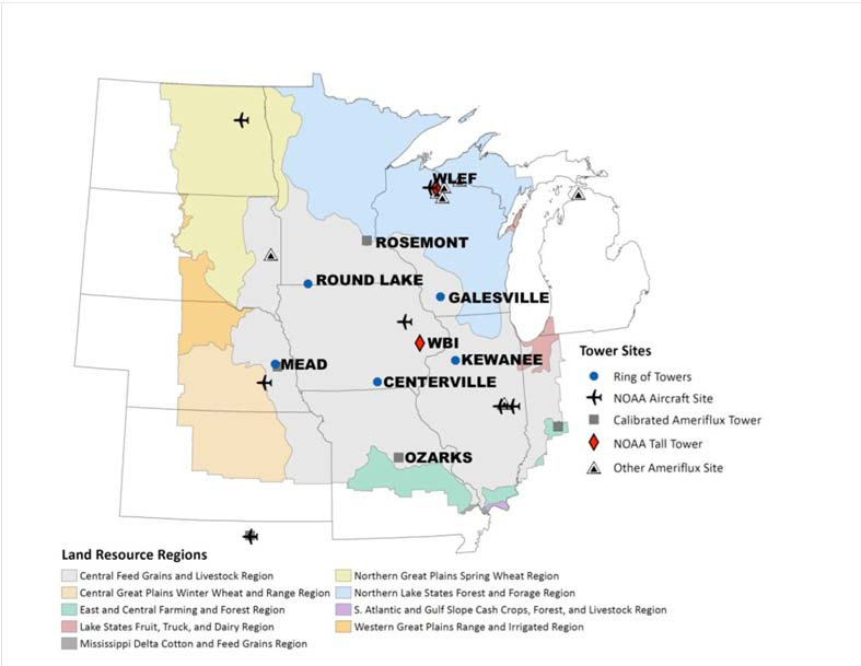
Figure 1. Map of MCI domain located in the U.S. Upper Midwest. Source: Schuh et al. (2013).

Authors:

Contact	Email
Schuh, Andrew E.	aschuh@kiwi.atmos.colostate.edu
Lauvaux, Thomas	tul5@psu.edu
Ogle, Stephen M.	stephen.ogle@colostate.edu
Davis, Kenneth J.	kjd10@psu.edu
Denning, A. Scott	scott.denning@colostate.edu
Miles, Natasha L.	nmiles@met.psu.edu
Richardson, Scott J.	srichardson@psu.edu
Uliasz, Marek	marek.uliasz@colostate.edu

Contact

Schuh, Andrew E.

aschuh@kiwi.atmos.colostate.edu

Lauvaux, Thomas

tul5@psu.edu

Ogle, Stephen M.

stephen.ogle@colostate.edu

Davis, Kenneth J.

kjd10@psu.edu

Denning, A. Scott

scott.denning@colostate.edu

Miles, Natasha L.

nmiles@met.psu.edu

Richardson, Scott J.

srichardson@psu.edu

Uliasz, Marek

marek.uliasz@colostate.edu

2. Data Description:

The NEE estimates are provided in two NetCDF files, one for each inversion system. Boundary CO2 inflow data are provided in three comma-separated-format files. The CSU inversion system used two versions of boundary CO2 inflow data, with one version using CarbonTracker CO2 (a modeling system to keep track of global CO2 sources and sinks) and the other version using bias-corrected CarbonTracker CO2 (bias-corrected with GlobalView CO2 data, a product of the Cooperative Atmospheric Data Integration Project).

2.1. Spatial Coverage

Site: U.S. Upper Midwest

Site Boundaries: (All latitude and longitude given in decimal degrees)

Site (Region)	Westernmost Longitude	Easternmost Longitude	Northernmost Latitude	Southernmost Latitude
U.S. Upper Midwest	-105	-81	50	36

Site (Region)

Westernmost Longitude

Easternmost Longitude

Northernmost Latitude

Southernmost Latitude

U.S. Upper Midwest

-105

-81

2.2. Spatial Resolution

The NEE estimates from both inversion systems included in this data set have a spatial resolution of 0.5 by 0.5-degree. The PSU inversion results were originally produced at a 20-km by 20-km resolution grid over a subset of the MCI region (Figure 2.B). The CSU inversion results were originally produced on a superset of the MCI, with a 40-km by 40-km grid over the MCI and a 200-km grid continentally (Figure 2.A).

Both native inversion results were on polar stereographic projections with different pole points within the MCI. The grid was then reprojected to a geographic lat/lon grid of 0.5 by 0.5-degree resolution using an area-weighted method. The following bullets briefly describe the reprojection process:

Create the target geographic lat/lon grid of 0.5 by 0.5-degree resolution as polygons (called GRID1)
Create the native polar stereographic grid for CSU or PSU inversion system correspondingly as polygons (called GRID2)
Reproject the set of polygons defined by GRID2 from polar stereographic projection to geographic lat/lon projection (called GRID2-lat/lon)
In R, use General Polygon Clipper library of the PBSmapping package to compare each polygon from GRID1 to each ploygon from GRID2-lat/lon, thereby building a matrix capable of converting results in GRID1 to GRID2-lat/lon. This process was applied to both “mean” and “variance” variables coming out of the inversions.

2.3. Temporal Coverage

Even though both the CSU and PSU inversion data files provided in this data set cover almost the whole year of 2007, the PSU inversion didn’t start until June of 2007 The PSU inversion used a “360 day” calendar, which assumes 30 days in each month and the last day of 2007 is Dec. 30th. The CSU inversion used a regular, or Gregorian, calendar. The exact temporal coverage of NEE estimates from CSU inversion is from 2007-01-01T00:00:00Z to 2007-12-30T12:59:59Z. The exact temporal coverage of NEE estimates from PSU inversion is from 2007-06-01T00:00:00Z to 2007-12-30:T23:59:59Z.

2.4. Temporal Resolution

The time resolution of the model results are explicitly stated in the NetCDF file metadata. The CSU inversion technique is a weekly sequential Bayesian batch inversion providing optimized daytime total respiration and gross primary production (GPP) on a weekly (7-day) time scale. The PSU inversion technique is a weekly sequential Bayesian batch inversion providing optimized estimates of daytime NEE and nighttime NEE on a 7.5-day time scale.

2.5. Data File Information

The inversion results are provided in two NetCDF version 4 files, one file from the CSU inversion system and the other from the PSU inversion system. Flux terms (NEE) are either 7-day summed (CSU) or 7.5-day summed (PSU) for means as well as covariances. Units are given as “grams of Carbon” but might be more properly interpreted as “grams of Carbon per inversion cycle”. The time given for the dimension of the fluxes represents the middle the summed NEE time step. The time_bnds variable represents the start and end of each summed NEE time step. See file details below.

2.5.1 CSU Inversion

File Name: CSU_RAMS_2007.1000KM.0.20SD.wr2aTF.111412.nc4

File Details:

netcdf CSU_RAMS_2007.1000KM.0.20SD.wr2aTF.111412 {
dimensions:
nv=2
lon = 48 ;
lat = 28 ;
time = UNLIMITED ; // (52 currently)
gridcell = 1344 ;
cov_label_nchar = 15 ;
cov_dim_names = 1344 ;

variables:
double lat_bnds (lat, nv) ;
    lat_bnds:units = "degrees_north" ;
double lon_bnds (lon, nv) ;
    lon_bnds:units = "degrees_east" ;
double time (time) ;
    time:bounds = "time_bnds" ;
    time:calendar = "standard" ;
    time:long_name = "time" ;
    time:units = "hours since 2007-01-01 00:00:00" ;
double time_bnds(time, nv) ;
    time_bnds:calendar = "standard" ;
    time_bnds:units = "hours since 2007-01-01 00:00:00" ;
double lon (lon) ;
    lon:units = "degrees_east" ;
    lon:long_name = "lon" ;
    lon:bounds = "lon_bnds" ;
double lat (lat) ;
    lat:units = "degrees_north" ;
    lat:long_name = "lat" ;
    lat:bounds = "lat_bnds" ;
float Prior_Mean_NEE (time, lat, lon) ;
    Prior_Mean_NEE:units = "grams C" ;
    Prior_Mean_NEE:_FillValue = 1.e+30f ;
float Posterior_Mean_NEE (time, lat, lon) ;
    Posterior_Mean_NEE:units = "grams C" ;
    Posterior_Mean_NEE:_FillValue = 1.e+30f ;
int gridcell (gridcell) ;
    gridcell:units = "index" ;
    gridcell:long_name = "gridcell" ;
float Posterior_Covariance_NEE (time, gridcell, gridcell) ;
    Posterior_Covariance_NEE:units = "(grams C)^2" ;
    Posterior_Covariance_NEE:_FillValue = 1.e+30f ;
int cov_label_nchar (cov_label_nchar) ;
    cov_label_nchar:long_name = "cov_label_nchar" ;
int cov_dim_names (cov_dim_names) ;
    cov_dim_names:long_name = "cov_dim_names" ;
char Posterior_Covariance_Labels_rows (cov_dim_names, cov_label_nchar) ;
char Posterior_Covariance_Labels_cols (cov_dim_names, cov_label_nchar) ;}

CSU Inversion Boundary Inflow

File Name: CSU_inversion_boundary_inflow.csv

File Details:

This file contains boundary inflow conditions used for tower CO2 concentrations for the CSU inversion. The boundary inflow conditions were created by convolving boundary “footprints”, produced via an LPDM model and the RAMS meteorology model, with CarbonTracker global optimized CO2 from CT2009. See Table 2 in Section 5 for tower characteristics. This represents the mass of CO2 that enters the CSU inversion region and is bound for the observing tower for the given convolving time period (3 hours).

Data User’s Note: This data file contains boundary inflow conditions at 19 towers (Table 2). Also, observations from 3 towers (Martha's Vineyard, Canaan Valley, and Erie, Colorado) were investigated but not used explicitly in the CSU inversion due to significant variability over short time periods.

TIME: Time is given in DOY since 2007-01-01T00:00:00Z (UTC). Each time value represents the end of a 3-hour sampling period.

Column Headings: Site Codes for the 19 towers that were considered in the CSU inversion. See Table 2 in Section 5 for Site characteristics.

VARIABLE:Values reported for each tower site are CO2 in ppm. Missing value = -999. Data User’s Note: The file CSU_inversion_boundary_inflow.csv contains these time series. The first 10 days are missing because of the 10 day integration time on the inversion makes the first 10 days data useless to the inversion. The last 2 days were omitted for ease of processing.

Sample Data Records:

TIME,amt,bao,ce,cl,cv,fd,gv,kw,lef,ll,me,mm,mo,mv,rl,rm,si,wbi,wkt Decimal_time_DOY,ppm,ppm,ppm,ppm,ppm,ppm,ppm,ppm,ppm,ppm,ppm,ppm,ppm,ppm,ppm,ppm,ppm,ppm,ppm
0.125,-999,-999,-999,-999,-999,-999,-999,-999,-999,-999,-999,-999,-999,-999,-999,-999,-999,-999,-999
0.25,-999,-999,-999,-999,-999,-999,-999,-999,-999,-999,-999,-999,-999,-999,-999,-999,-999,-999,-999
-999 -999 -999 -999 -999 -999 -999 -999 -999 -999 -999 -999 -999 -999 -999 -999 -999 -999 -999
...

13.125,387.428626279478,386.29611615051,387.012229191903,389.198762651905,
385.55062506417,387.089620726418,387.920719497968,386.95618834757,
387.562899333528,388.205513372276,385.824002257556,387.405827703058,386.533256797187, 386.022426584577,387.907345653355,387.603264020641,386.617746931783,386.989790935715, 386.292788413719
...
13,-999,-999,-999,-999,-999,-999,-999,-999,-999,-999,-999,-999,-999,-999,-999,-999,-999,-999,-999
13.25,,387.4286263,386.2961162,387.0122292,389.1987627,385.5506251,387.0896207,387.9207195
386.9561883,387.5628993,388.2055134,385.8240023,387.4058277,386.5332568,386.0224266,
387.9073457,387.603264,386.6177469,386.9897909,386.2927884
13.25,387.4100381,386.3883325,387.3560563,388.9533465,385.5707711,387.1902286,387.9055843
386.924956,387.5137132,388.1409477,386.0770888,387.4660232,386.4188389,386.051756,387.8850804
387.5324959,386.7342267,386.7466399,386.0180636
...
363,388.1306343,387.2435233,388.0919988,388.1234045,388.3436178,388.833934,389.4429689,
389.3218636,390.0842024,386.2681417,385.949746,388.1158971,388.1711821,387.6807122,
387.9243415,388.398274,387.1969114,388.2438576,388.6772685
363.125,-999,-999,-999,-999,-999,-999,-999,-999,-999,-999,-999,-999,-999,-999,-999,-999,-999,-999,-999
...

CSU Inversion Boundary Inflow for GlobalView (Bias-corrected CT Inflow)

File Name: CSU_inversion_boundary_GV_inflow_corrected.csv

File Details:

This file contains a different version of boundary inflow conditions used for tower CO2 concentrations for the CSU inversion. The purpose is to test boundary inflow sensitivity for the CSU continental inversions. The boundary inflow conditions were created by convolving boundary “footprints”, produced via an LPDM model and the RAMS meteorology model, with CarbonTracker global optimized CO2 from CT2009 bias-corrected using GlobalView CO2 product. The bias-correction was conducted by subtracting a 3-week moving average of the difference between CarbonTracker optimized CO2 and Globalview CO2, from the CarbonTracker optimized CO2. See Table 2 in Section 5 for tower characteristics. This represents the mass of CO2 that enters the CSU inversion region and is bound for the observing tower for the given convolving time period (3 hours).

Data User’s Note: This data file contains boundary inflow conditions at 19 towers (Table 2). Any observation for which the “a-prior” model-data mismatch was greater than 40 ppm was not used in the CSU inversion. Also, observations from 3 towers (Martha's Vineyard, Canaan Valley, and Erie Colorado) were investigated but not used explicitly in the CSU inversion due to significant variability over short time periods.

TIME: Time is given in decimal DOY since 2007-01-01T00:00:00Z (UTC). Each time value represents the end of a 3-hour sampling period.

Column Headings: Site Codes for the 19 towers that were considered in the CSU inversion. See Table 2 in Section 5 for Site characteristics.

VARIABLES: Values reported for each tower site are CO2 in ppm. Missing value = -999.

Sample Data Records:

2.5.2 PSU Inversion

File Name: PSU_WRF_2007_20KM.013013.nc4

Data User’s Note: Due to measurements from the MCI Ring 2 towers not starting until June 2007, no Posterior_Mean_NEE adjustments were performed during the January through May period. The values for Prior_Mean_NEE and the Posterior_Mean_NEE parameters are equal.

File Details: Header of NetCDF file

netcdf PSU_WRF_2007_20KM.013013 {
dimensions:
    nv=2
    lon = 48 ;
    lat = 28 ;
    time = UNLIMITED ; // (48 currently)
    gridcell = 1344 ;
    cov_label_nchar = 15 ;
    cov_dim_names = 1344 ;

variables:
double lat_bnds (lat, nv) ;
    lat_bnds:units = "degrees_north" ;
double lon_bnds (lon, nv) ;
    lon_bnds:units = "degrees_east" ;
double time (time) ;
    time:bounds = "time_bnds" ;
    time:calendar = "360_day" ;
    time:long_name = "time" ;
    time:units = "hours since 2007-01-01 00:00:00" ;
double time_bnds (time, nv) ;
    time_bnds:calendar = "360_day" ;
    time_bnds:units = "hours since 2007-01-01 00:00:00" ;
double lon (lon) ;
    lon:units = "degrees_east" ;
    lon:long_name = "lon" ;
    lon:bounds = "lon_bnds" ;
double lat (lat) ;
    lat:units = "degrees_north" ;
    lat:long_name = "lat" ;
    lat:bounds = "lat_bnds" ;
float Prior_Mean_NEE (time, lat, lon) ;
    Prior_Mean_NEE:units = "grams C" ;
    Prior_Mean_NEE:_FillValue = 1.e+30f ;
float Posterior_Mean_NEE (time, lat, lon) ;
    Posterior_Mean_NEE:units = "grams C" ;
    Posterior_Mean_NEE:_FillValue = 1.e+30f ;
int gridcell (gridcell) ;
    gridcell:units = "index" ;
    gridcell:long_name = "gridcell" ;
float Posterior_Covariance_NEE (time, gridcell, gridcell) ;
    Posterior_Covariance_NEE:units = "(grams C)^2" ;
    Posterior_Covariance_NEE:_FillValue = 1.e+30f ;
int cov_label_nchar (cov_label_nchar) ;
    cov_label_nchar:long_name = "cov_label_nchar" ;
int cov_dim_names (cov_dim_names) ;
    cov_dim_names:long_name = "cov_dim_names" ;
char Posterior_Covariance_Labels_rows (cov_dim_names, cov_label_nchar) ;
char Posterior_Covariance_Labels_cols (cov_dim_names, cov_label_nchar) ;}

Data User Note for Inversion NetCDF Files:

The covariance matrix has several possible orderings depending upon which way the georeferenced grid was converted to a vector. The fields Posterior_Covariance_Labels_rows and Posterior_Covariance_Labels_cols specify the index/order of the 2-d matrix grid cells as converted to the 1-d vector for the purposed of calculating Posterior_Covariance_NEE. The Posterior_Covariance_Labels_rows and Posterior_Covariance_Labels_cols fields are populated with the latitude and longitude centroid values corresponding to that 2-d matrix grid cell as a text string. For example:

Posterior_Covariance_Labels_rows = "36.25 -104.75", “36.75 -104.75", "37.25 -104.75", …
Posterior_Covariance_Labels_cols = "36.25 -104.75", "36.75 -104.75", "37.25 -104.75", …

In this case, conversion started with the upper left corner grid cell and proceeded across that row and then back to the left-most grid cell of the next row, etc.

PSU Inversion Boundary Inflow

File Name: PSU_inversion_boundary_inflow.csv

File Details:

This file contains boundary inflow conditions used for tower CO2 concentrations for the PSU inversion. The boundary inflow conditions were created by convolving boundary “footprints”, produced via an LPDM model and the WRF meteorology model, with CarbonTracker global optimized CO2 from CT2009. A weekly correction of the boundary inflow was applied to CT2009 by adjusting the hourly concentrations with CO2 observations from the NOAA aircraft program. 4 aircraft sites were used to correct for weekly biases: Homer, Illinois (HIL), Bondville, Illinois (AAO), LEF, and Beaver Crossing, Nebraska (BNE). Data are available at: http://www.esrl.noaa.gov/gmd/ccgg/aircraft/. See Table 2 in Section 5 for tower characteristics. This represents the mass of CO2 that enters the PSU inversion region and is bound for the observing tower for the given convolving time period (1 hour). This file contains 1-hour boundary inflow for 8 towers that were considered in the PSU inversion. See Table 2 in Section 5 for tower characteristics. This represents the mass of CO2 that enters the MCI from outside the region. Anyone who wants to reproduce the inversion results can directly use these values.

Data User’s Note: The first 5 months, through DOY 150, are filled with missing values (-999) because the measurements from the MCI Ring 2 towers did not start until June 2007. The last day was omitted for ease of processing.

TIME: Time is given in decimal DOY since 2007-01-01T00:00:00Z (UTC). Each time value represents the end of a 3-hour sampling period.

Column Headings: Site Codes for the 19 towers that were considered in the CSU inversion. See Table 2 in Section 5 for Site characteristics.

VARIABLES: Values reported for each tower site are CO2 in ppm. Missing value = -999. Data User’s Note: The file CSU_inversion_boundary_inflow.csv contains these time series. The first 10 days are missing because of the 10 day integration time on the inversion makes the first 10 days data useless to the inversion. The last 2 days were omitted for ease of processing.

Sample Data Records

TIME,cv,kw,rl,mm,gv,mo,wbi,lef Decimal_time_DOY,ppm,ppm,ppm,ppm,ppm,ppm,ppm,ppm
0,-999,-999,-999,-999,-999,-999,-999,-999 0.04167,-999,-999,-999,-999,-999,-999,-999,-999
...
150.91667,-999,-999,-999,-999,-999,-999,-999,-999
150.95833,-999,-999,-999,-999,-999,-999,-999,-999
151,379.95685,379.95685,379.95685,379.95685,379.95685,379.95685,379.95685,379.95685
151.04167,379.95685,379.95685,379.95685,379.95685,379.95685,379.95685,379.95685,379.95685
151.08333,379.95685,379.95685,379.95685,379.95685,379.95685,379.95685,379.95685,379.95673
…
363.91666,392.03375,382.97314,392.06131,391.82928,388.84036,392.01694,382.83453,387.6066
363.95834,392.65009,384.73776,392.0813,392.03238,388.91458,392.43805,384.68784,387.45963
364,-999,-999,-999,-999,-999,-999,-999,-999
364.04166,-999,-999,-999,-999,-999,-999,-999,-999
364.08334,-999,-999,-999,-999,-999,-999,-999,-999

3. Data Application and Derivation:

This data product contributes to a multidisciplinary research program to obtain scientific understanding of North America's carbon sources and sinks and of changes in carbon stocks needed to meet societal concerns and to provide tools for decision makers. The data were generated as part of the NACP Mid-Continent Intensive (MCI) experimental campaign.

The data set contributes to an effort to resolve net CO2 exchange in the Mid-Continent Region of North America. The results are used to compare and reconcile "top-down" inverse modeling (this data set) and "bottom-up" inventory-based approaches.

As discussed in Schuh et al. (2013) one of the primary objectives of the intensive campaign was to investigate the ability of atmospheric inversion techniques to use highly calibrated CO2 mixing ratio data to estimate CO2 flux over the major croplands of the United States by comparing the results to an inventory of CO2 fluxes. Statistics from densely monitored crop production, consisting primarily of corn and soybeans, provided the backbone of a well-studied bottom-up inventory flux estimate that was used to evaluate the atmospheric inversion results. Estimates were compared to the inventory from three different inversion systems, representing spatial scales varying from high resolution mesoscale (PSU), to continental (CSU) and global (CarbonTracker), coupled to different transport models and optimization techniques. Figure 2 show the results of these comparisons.

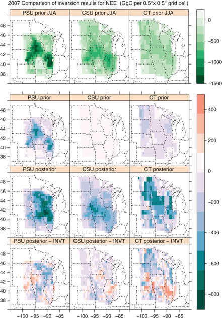
graphic of CO2 inversion model results

Figure 2. (Schuh et al. (2013), Figure 5) Each panel name is composed of the following (i) inversion model, (ii) 2007 for annual total or JJA2007 for June/July/August sum, and (iii) ‘pr’ for a priori and ‘post’ for posterior flux. A priori annual 2007 NEE estimates are shown in middle row with posterior annual 2007 NEE estimates shown in the bottom row. The bottom row consists of differences between the inversion models and the inventory (INVT). PSU inversion is based on SiB3-CROP offline prior with residual 109 TgC harvest sink. CSU inversion is also based on same prior (and underlying seasonality), but with residual harvest sink balanced by respiration annually to induce net zero NEE and uses GlobalView bias-corrected CT inflow. The top row shows the June/July/August total NEE for each prior flux which is indicative of the spatial signal of strong summer crop carbon drawdown. A few grid cell values were truncated at the bounds of the color bar for visualization purposes. Multiplying fluxes by 0.45 gives approximate conversion into grams per square meter.

4. Quality Assessment:

The atmospheric CO2 inversion process creates an explicit variance based upon Gaussian assumptions inherent in both the PSU and CSU inversion schemes. Additional uncertainty can arise as a function on errors in transport and boundary inflow of CO2, both of which are generally considered fixed and “known”. See Schuh et al. (2013) and Lauvaux et al. (2012a) for more details.

5. Data Acquisition Materials and Methods:

The goal of this study was to provide time-varying mean and covariance estimates for a set of spatial CO₂ fluxes covering the MCI region that are consistent with observed CO₂ concentrations. The main differences among the inversion frameworks are summarized in the table below.

Table 1. Comparison of inversion model components (Source: Schuh et al., 2013)

Component	CSU (SiB-RAMS-LPDM)	PSU (WRF-LPDM)	CarbonTracker (results not included in this data set)
Inversion method	Synthesis Bayesian	Synthesis Bayesian	Ensemble Kalman filter
Transport	BRAMS 3.2¹	WRF-Chem	TM5
Land surface model²	SiB3-CROP	NOAH	TESSEL
A priori CO₂ fluxes/photosynthesis model type	SiB3-CROP (Farquhar)	SiB3-CROP (Farquhar)	CASA (LUE)
Domain	Continental (North America)	Regional	Global
Transport resolution	40-km	10-km	3 x 2-deg (1 x - deg nest)
Inversion resolution	40-km/200-km nest	20-km	Ecoregions (Olsen)
Boundary CO₂	CarbonTracker and GlobalView	Aircraft-corrected CarbonTracker	None (global)

Component

CSU (SiB-RAMS-LPDM)

PSU (WRF-LPDM)

CarbonTracker
(results not included in this data set)

Inversion method

Synthesis Bayesian

Ensemble Kalman filter

Transport

BRAMS 3.2¹

WRF-Chem

TM5

Land surface model²

SiB3-CROP

NOAH

TESSEL

A priori CO₂ fluxes/photosynthesis model type

SiB3-CROP (Farquhar)

CASA (LUE)

Domain

Continental (North America)

Regional

Global

Transport resolution

40-km

10-km

3 x 2-deg (1 x - deg nest)

Inversion resolution

40-km/200-km nest

20-km

Ecoregions (Olsen)

Boundary CO₂

CarbonTracker and GlobalView

Aircraft-corrected CarbonTracker

None (global)

Notes:

¹BRAMS 3.2 was used as the basis for the transport model but the code has undergone numerous changes, fixes, and improvements over the last decade at Colorado State University.

²The LSM used to drive the meteorology in the inversion, not necessary consistent with the LSM used to generate the a priori CO2 fluxes.

BRAMS = Brazilian Regional Atmospheric Modeling System.

WRF-Chem = Weather Research and Forecasting (WRF) model coupled with Chemistry.

TM5 =two-way nested global atmospheric chemistry-transport ZOOM model.

SiB3-CROP = Simple Biosphere model (SiB) with phenology-based crop module (Lokupitiya et al., 2009). The photosynthesis in SiB follows the Farquhar approach (Farquhar et al., 1980).

CASA (LUE) = CASA-GFEDv2 model runs of the Carnegie-Ames Stanford Approach (CASA) biogeochemical model, which employs a light use efficiency (LUE) photosynthesis model based upon AVHRR NDVI and year-specific weather.

NOAH = the NCEP Community NOAH Land-Surface Model [N: National Centers for Environmental Prediction (NCEP); O: Oregon State University (Dept of Atmospheric Sciences); A: Air Force (both AFWA and AFRL - formerly AFGL, PL); H: Hydrologic Research Lab - NWS (now Office of Hydrologic Dev -- OHD)].

TESSEL = Tiled ECMWF Scheme for Surface Exchanges over Land.

Mid-Continent Intensive Region. The U.S. upper Midwest (Figure 1 above) was the region selected for the MCI because of its uncomplicated terrain and because the dominant crop ecosystems are extensively documented. The region is primarily agricultural, with cropland and grassland being the dominant vegetation types, but has forest cover in the southern and especially northern portions of the region (U.S. Geological Survey Land Cover Institute, 2010; see http://landcover.usgs.gov). Corn and soybeans are the dominant crops; in Iowa, the area planted with these crops is 52% and 41% of the total agricultural area, respectively [U.S. Department of Agriculture, National Agricultural Statistics Service (USDA, NASS), 2010].

Spatial Domain and Resolution for Inversions. The PSU inversion was run on a rectangular domain which overlapped portions of the non-rectangular MCI domain. Consequently, estimates for the PSU inversion were lacking for some areas in the MCI and were provided for some areas not in the MCI. As a result, we often present estimates for two areas, (i) the full MCI and (ii) the intersection of the PSU inversion domain and the MCI, which covers approximately 71% of the MCI domain. The CSU domain consisted of most of North America and extended out into the oceans to the east and west.

The CSU inversion domain consisted of a grid of 200-km by 200-km grid cells over most of North America with higher resolution grid of 40-km by 40-km grid cells over the MCI, covering the entire underlying transport grid. The PSU inversion domain consisted of a grid of 20-km by 20-km grid cells over their transport grid. Both domains are shown in Figure 3.

spatial domain

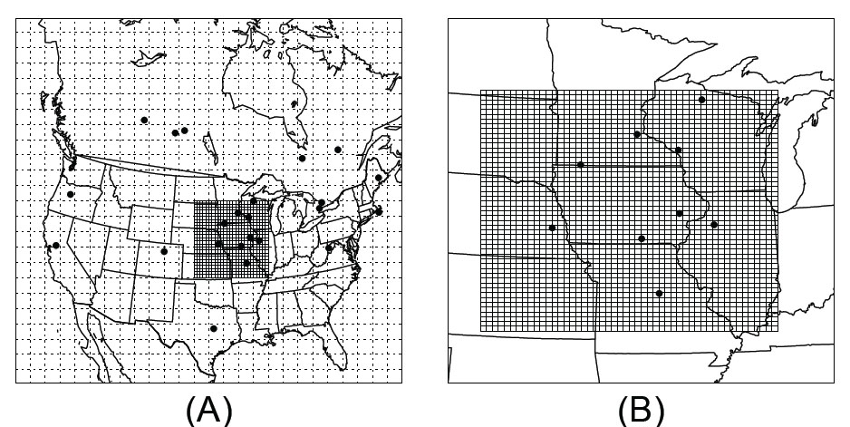
Figure 3. Inversion domains shown in native polar stereographic projections. Left panel (A) shows nested inversion grid with coarser grid at 200-km by 200-km and fine grid over MCI at 40-km by 40-km. Right panel (B) shows high resolution 20-km by 20-km grid for PSU inversion system. Source: Schuh et al. (2013).

Optimization and Temporal Resolution. The CSU inversion technique is a weekly sequential Bayesian batch inversion providing optimized total respiration (OPT_TRESP) and gross primary production (OPT_GPP) on a weekly time scale at 40-km by 40-km over the MCI and 200-km continentally. A priori total respiration (TRESP) and gross primary production (GPP) are independently ‘corrected’ via regression factors, β_TRESP and β_GPP applied to the a priori fluxes. The PSU inversion technique is a weekly sequential Bayesian batch inversion providing optimized estimates of daytime NEE and nighttime NEE on a 7.5 day time scale at 20-km by 20-km spatial resolution. In contrast to optimizing ‘correction factors’ as the CSU inversion does, the PSU inversion directly optimizes the fluxes. See Schuh et al. (2013) for details.

The PSU inversion was run from June through December of 2007 due to its domain and dependency on the Ring data which began in June 2007. Where annual totals were required, a priori CO2 distributions were used. This is not likely to be a critical limitation to the comparison, however, because the dominant fluxes are occurring between June and August. In addition, the PSU inversion uses an a priori annual flux consistent with the removal of harvested crops and thus one would not expect large differences in the optimization during January through May, when respiration is the primary CO2 flux. The CSU inversion results contains prior flux results for the first three weeks of the year due to a lack of meteorological driving data from the end of 2006 which was needed to interpret early January 2007 results.

Inversion Process

A schematic of the inversion process is shown in Figure 4. Details are described below.

schematic of inversion process

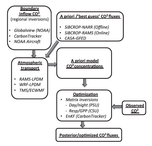
Figure 4. Flowchart of atmospheric inversion process. Source: Schuh et al. (2013).

Boundary Inflow CO2.The boundary inflow for the CSU inversion results was derived by integrating Lagrangian particles exiting the domain over both the GlobalView CO2 curtain product (Arlyn Andrews, NOAA-ESRL) and the NOAA CarbonTracker optimized CO2 product (CT2009). A 3-month moving average of differences between the two products were used to bias correct the NOAA CT product, which was then used as the inflow estimate to each tower. The PSU inversion also utilizes optimized CT CO2 bias corrected with routine NOAA aircraft flights near their domain boundaries (Lauvaux et al., 2012b). See Schuh et al. (2013) and data files for details.

CSU Inversion Boundary Conditions:

The boundary conditions used for tower CO2 concentrations for the CSU inversion in this data set are described in Schuh et al. (2013). The boundary conditions were created by convolving boundary "footprints", produced via an LPDM model and the RAMS meteorology model, with CarbonTracker global optimized CO2 from CT2009. The domain ran from -4e6,4e6 (horiz) and -2.4e6,2.4e6 (vertical), centered on the (0,0) point of the projection given [proj4 projection, "+proj=sterea +lat_0=48d00N +lon_0=98d00W +k_0=1 +x_0=0 +y_0=0 +ellps=WGS84", (https://trac.osgeo.org/proj/)]. Thus the inflow was created where the 2D boundary edge intersects the Eulerian CarbonTracker grid. The file CSU_inversion_boundary_inflow.csv contains these time series. The first 10 days are missing because of the 10 day integration time on the inversion makes the first 10 days data useless to the inversion. The last 2 days were omitted for ease of processing.

The file CSU_inversion_boundary_inflow.csv contains these time series. The first 10 days are missing because of the 10 day integration time on the inversion makes the first 10 days data useless to the inversion. The last 2 days were omitted for ease of processing.

The file CSU_inversion_boundary_GV_inflow_corrected.csv was created by an additional convolving of the boundary footprint files with the globalview boundary curtain file (Arlyn Andrews, ESRL-NOAA). In particular, the original CarbonTracker boundary inflow time series were bias-corrected by (1) calculating the three-week moving average of CO2 of CarbonTracker (for each tower) and the three-week moving average of CO2 from the GlobalView boundary curtain, and (2) removing the difference of these two time series from the original CarbonTracker inflow. In some sense, this maintains the synoptic dynamics in the optimized CarbonTracker CO2 fields while maintaining the longer term CO2 averages given by the GlobalView boundary curtain product.Boundary contributions at towers are provided for the 19 towers listed in Table 2.

PSU Inversion Boundary Conditions:

The boundary conditions used for tower CO2 concentrations for the PSU inversion are described in Schuh et al. (2013). The boundary conditions were created by using CarbonTracker (version 2009) CO2 mixing ratios coupled to the Weather Research and Forecasting model, and corrected from weekly biases using CO2 mixing ratio observations from the NOAA aircraft program (Lauvaux et al., 2012). The domain for the PSU inversion was a 100 x 100 10-km projected domain using a polar stereographic projection, "+proj=sterea +lat_0=41.3N +lon_0=92.9W +k_0=1 +x_0=0 +y_0=0 +ellps=WGS84". Thus the inflow was created where the 2D boundary edge intersects the Eulerian CarbonTracker grid. The PSU_boundary_inflow.csv file contains the time series data. The first 5 months are missing (value = -999) because the deployment of MCI towers did not start until June 2007. The last day was omitted for ease of processing. Boundary contributions in the PSU_boundary_inflow.csv file are given for 8 towers identified in Table 2.

The PSU_boundary_inflow.csv file contains the time series data. The first 5 months are missing (value = -999) because the deployment of MCI towers did not start until June 2007. The last day was omitted for ease of processing.

Boundary contributions in the PSU_boundary_inflow.csv file are given for 8 towers identified in Table 2.

Table 2. Towers: Name/location, longitude, latitude, height above ground level (m)

Site Code	Full Name	Latitude (degrees N)	Longitude (degrees W)	Elevation (m AMSL)	CSU boundary condition towers	PSU boundary condition towers
CE	Centerville, Iowa	40.7919	-92.8775	110	Yes	Yes
GV	Galesville, Wisconsin	44.0910	-91.3382	122	Yes	Yes
KW	Kewanee, Illinois	41.2762	-89.9724	140	Yes	Yes
MM	Mead, Nebraska	41.1386	-96.4559	48	Yes	Yes
RL	Round Lake, Minnesota	43.5263	-95.4137	110	Yes	Yes
MO	Missouri Ozarks, Missouri	38.7441	-92.2000	219	Yes	Yes
RM	Rosemount, Minnesota	44.6886	-93.0728	200	Yes
Amt	Argyle, ME	-68.68	45.03	107	Yes
BAO	Erie, CO	-105.01	40.05	300	Yes
CL	Candle Lake, SK	-104.8833	53.9833	30	Yes
CV	Canaan Valley, WV	-104.8833	53.98333	7	Yes
FD	Fraserdale, ON	-80.4333	49.8833	40	Yes
LEF	Park Falls, WI	-90.27	45.95	396	Yes	Yes
LL	Lac Labiche, AB	-111.55	54.95	10	Yes
ME	Metolius, OR	-121.55716	82.45	32	Yes
MV	Martha's Vineyard, MA	-70.52	41.33	10	Yes
SI	Sable Island, NB	-59.9833	43.9333	25	Yes
WBI	West Branch, IA	-91.35286	41.72478	379	Yes	Yes
WKT	Moody, TX	-97.33	31.32	107	Yes

Atmospheric Transport. The WRF-Chem was used for transport by the PSU inversion system at a resolution of 10-km by 10-km. A CSU version of the Brazilian Regional Atmospheric Modeling System (BRAMS) was used for transport in the CSU model at a resolution of 40-km by 40-km.

The Lagrangian particle model LPDM is used by both PSU and CSU. It effectively acts as a transport adjoint (i.e. ‘inverse’) by diagnosing turbulent motions in the atmosphere as a function of high time resolution fields of zonal and meridional winds, potential temperature, and turbulent kinetic energy output from a parent mesoscale model. This allows for the creation of a Jacobian matrix representing the partial derivatives of CO2 concentration (at a fixed location) with respect to the surrounding fluxes of CO2. The details of the Lagrangian model that produces the particle movements from the parent mesoscale model can be found in Uliasz (1994). Further details on this technique can be seen in the Supporting Information, Appendix D1 of Schuh et al. (2013).

A priori CO2 Fluxes. The inversions use a priori CO2 flux distributions that are Gaussian in nature and are thus composed of mean and covariance information.

Means: The a priori flux assumptions for the CSU and PSU regional models are based on the Simple Biosphere model with a phenology-based crop module (SiB-CROP) (Lokupitiya et al., 2009). The photosynthesis in SiB follows the Farquhar approach (Farquhar et al., 1980). SiB-CROP was used in two ways. First, hourly CO2 fluxes were calculated from offline runs of the model driven by North American Regional Reanalysis meteorological data, at 40-km by 40-km resolution and 10-km by 10-km resolution, respectively, with three sub-gridscale landcover patches for each configuration. Secondly, the CSU model also ran test cases in which the SiB-CROP model was run in coupled-mode inside of BRAMS in an effort to provide consistency between the modeled CO2 fluxes and the meteorological data.

Covariances: For the CSU inversion, a priori covariance matrices for the multiplicative biases on GPP and TRESP were formed by constructing isotropic exponential spatial covariance structures over North America with decorrelation length scales of 500 and 1000-km and scaling them to 0.2, which amounts to standard deviations of 20% on GPP and TRESP. See Supporting Information, Appendix A4 of Schuh et al. (2013) for more information.

A priori covariance assumptions for the PSU inversion included smaller decorrelation length scales (exponential covariance) of approximately 300-km, compared to the CSU inversion which generally employed 500 and 1000-km. The smaller decorrelation length scales of the PSU inversion were further decreased by modeling the covariance length scale as a function of ecosystem type, resulting in equivalent isotropic decorrelation length scales of approximately 100-km. The temporal correlations were calculated consistent with Lauvaux et al. (2009). See Supporting Information, Appendix A4 of Schuh et al. (2013) and Lauvaux et al. (2012b) for more information.

Observed CO2.The PSU and CSU inversions both used CO2 observations from a network of instrumented tall towers in the region [e.g., the PSU Ring 2 network (Miles et al., 2012) and Missouri Ozarks (Gu et al., 2006; 2008; 2012; Stephens et al., 2011)] while using slightly different data streams from NOAA tall towers at WLEF in Wisconsin and WBI in Iowa. The PSU inversion used data from 122 m at WLEF and 99 m at WBI to be consistent with the other tower heights (i.e., Ring 2 sites and Missouri Ozarks) while the CSU inversion used the highest levels for WLEF and WBI which are 396 and 379 m, respectively. The CSU inversion also used CO2 observations from tower sites outside of the PSU spatial domain. The full observational constraints for the PSU and CSU inversions are summarized in Table 3.

Table 3. CO2 Tower Observation Sites

Tower Site	Height (m)	Contact	PSU Inversion	CSU Inversion
Argyle, ME	107	A. Andrews, NOAA-ESRL	Outside domain	12:00–18:00 LST
Centerville, IA	110	N. Miles/S. Richardson, Penn State U	All hours	12:00–18:00 LST
Candle Lake, BC	30	D. Worthy, EnviroCanada	Outside domain	12:00–18:00 LST
Fraserdale, ON	40	D. Worthy, EnviroCanada	Outside domain	12:00–18:00 LST
Galesville, WI	122	N. Miles/S. Richardson, Penn State U	All hours	12:00–18:00 LST
Kewanee, IL	140	N. Miles/S. Richardson, Penn State U	All hours	12:00–18:00 LST
Park Falls, WI (WLEF)	122/396	A. Andrews, NOAA-ESRL	All hours (122 m)	12:00–18:00 LST (396 m)
Lac Labiche, AB	10	D. Worthy, EnviroCanada	Outside domain	12:00–18:00 LST
Metolius, OR	33	M. Goeckede/Beverly Law, Oregon State University	Outside domain	12:00–18:00 LST
Mead, NE	122	N. Miles/S. Richardson, Penn State U	All hours	12:00–18:00 LST
Missouri Ozarks, MO	30	N. Miles/S. Richardson, Penn State U	All hours	12:00–18:00 LST
Round Lake, MN	110	N. Miles/S. Richardson, Penn State U	All hours	12:00–18:00 LST
Sable Island, NS	25	D. Worthy, EnviroCanada	Outside domain	12:00–18:00 LST
West Branch, IA (WBI)	99/379	A. Andrews, NOAA-ESRL	All hours (99 m)	12:00–18:00 LST (379 m)
Moody, TX	457	A. Andrews, NOAA-ESRL	Outside domain	12:00–18:00 LST

Tower Site

Height (m)

Contact

PSU Inversion

CSU Inversion

Argyle, ME

107

A. Andrews, NOAA-ESRL

Outside domain

12:00–18:00 LST

Centerville, IA

110

N. Miles/S. Richardson, Penn State U

All hours

12:00–18:00 LST

Candle Lake, BC

D. Worthy, EnviroCanada

Outside domain

12:00–18:00 LST

Fraserdale, ON

D. Worthy, EnviroCanada

Outside domain

12:00–18:00 LST

Galesville, WI

122

N. Miles/S. Richardson, Penn State U

All hours

12:00–18:00 LST

Kewanee, IL

140

N. Miles/S. Richardson, Penn State U

All hours

12:00–18:00 LST

Park Falls, WI (WLEF)

122/396

A. Andrews, NOAA-ESRL

All hours (122 m)

12:00–18:00 LST (396 m)

Lac Labiche, AB

D. Worthy, EnviroCanada

Outside domain

12:00–18:00 LST

Metolius, OR

M. Goeckede/Beverly Law, Oregon State University

Outside domain

12:00–18:00 LST

Mead, NE

122

N. Miles/S. Richardson, Penn State U

All hours

12:00–18:00 LST

Missouri Ozarks, MO

N. Miles/S. Richardson, Penn State U

All hours

12:00–18:00 LST

Round Lake, MN

110

N. Miles/S. Richardson, Penn State U

All hours

12:00–18:00 LST

Sable Island, NS

D. Worthy, EnviroCanada

Outside domain

12:00–18:00 LST

West Branch, IA (WBI)

99/379

A. Andrews, NOAA-ESRL

All hours (99 m)

12:00–18:00 LST (379 m)

Moody, TX

457

A. Andrews, NOAA-ESRL

Outside domain

12:00–18:00 LST

Notes:

All towers used by PSU inversion were used by CSU inversion. Additional towers were used by CSU due to larger domain size. PSU inversion uses all hours but with different weightings for different times of day and therefore nocturnally collected data is usually weighted more weakly. See Lauvaux et al. (2012b).

6. Data Access:

This data set is available through the Oak Ridge National Laboratory (ORNL) Distributed Active Archive Center (DAAC).

Data Archive Center:

Contact for Data Center Access Information:
E-mail: uso@daac.ornl.gov
Telephone: +1 (865) 241-3952

7. References:

Denning, A.S., et al. 2005. Science implementation strategy for the North American Carbon Program: A Report of the NACP Implementation Strategy Group of the U.S. Carbon Cycle Interagency Working Group. U.S. Carbon Cycle Science Program, Washington, DC. 68 pp.

Farquhar, G.D., S. Von Caemmerer, and J.A. Berry. 1980. A biochemical model of photosynthetic CO₂ fixation in the leaves of C₃ species. Planta 149: 78-90. doi:10.1007/BF00386231

Lauvaux, T., O. Pannekoucke, C. Sarrat, F. Chevallier, P. Ciais, J. Noilhan, and P.J. Rayner. 2009. Structure of the transport uncertainty in mesoscale inversions of CO₂ sources and sinks using ensemble model simulations. Biogeosciences 6: 1089-1102. doi:10.5194/bg-6-1089-2009

Lauvaux, T., A.E. Schuh, M. Bocque, L. Wu, S. Richardson, N. Mile, and K.J. Davis. 2012a. Network design for mesoscale inversions of CO₂ sources and sinks. Tellus B, North America, 64, 17980. doi:10.3402/tellusb.v64i0.17980

Lauvaux, T., A.E. Schuh, M. Uliasz, S. Richardson, N. Miles, A E. Andrews, C. Sweeney, L.I. Diaz, D. Martins, P.B. Shepson, and K.J. Davis. 2012b. Constraining the CO₂ budget of the corn belt: exploring uncertainties from the assumptions in a mesoscale inverse system. Atmos. Chem. Phys. 12: 337–354. doi:10.5194/acp-12-337-2012

Lokupitiya, E., S. Denning, K. Paustian, I. Baker, K. Schaefer, S. Verma, T. Meyers, C.J. Bernacchi, A. Suyker, and M. Fischer. 2009. Incorporation of crop phenology in Simple Biosphere Model (SiBcrop) to improve land-atmosphere carbon exchanges from croplands. Biogeosciences 6: 969-986. doi:10.5194/bgd-6-1903-2009

Miles, N.L., S.J. Richardson, K.J. Davis, T. Lauvaux, A.E. Andrews, T.O. West, V. Bandaru, and E. R. Crosson. 2012. Large amplitude spatial and temporal gradients in atmospheric boundary layer CO₂ mole fractions detected with a tower‐based network in the U.S. upper Midwest. J. Geophys. Res. 117: G01019. doi:10.1029/2011JG001781

Schuh, A.E., T. Lauvaux, T.O. West, A.S. Denning, K.J. Davis, N. Miles , S. Richardson, M. Uliasz , E. Lokupitiya, D. Cooley, A. Andrews, and S. Ogle. 2013. Evaluating atmospheric CO₂ inversions at multiple scales over a highly inventoried agricultural landscape. Global Change Biology 19: 1424-1439. doi: 10.1111/gcb.12141

Uliasz, M. 1994. Lagrangian particle modeling in mesoscale applications. In: Environmental Modeling II (ed. Zannetti P), pp. 71–102. Computational Mechanics Publications, Southampton, UK.

U.S. Department of Agriculture, National Agricultural Statistics Service (USDA, NASS). 2010. Quick Stats Database [http://www.nass.usda.gov/Quick_Stats/]. Washington, D.C.

Wofsy, S.C., and R.C. Harriss. 2002. The North American Carbon Program (NACP). Report of the NACP Committee of the U.S. Interagency Carbon Cycle Science Program. U.S. Global Change Research Program, Washington, DC. 56 pp.

Summary:

Data and Documentation Access:

Data Citation:

Table of Contents:

1. Data Set Overview:

2. Data Description:

3. Data Application and Derivation:

4. Quality Assessment:

5. Data Acquisition Materials and Methods:

6. Data Access:

Data Archive Center:

7. References: