CMS: Forest Carbon Stocks, Emissions, and Net Flux for the Conterminous US: 2005-2010

This data set provides maps of estimated carbon in forests of the 48 continental states of the US for the years 2005-2010. Carbon (termed committed carbon) stocks were estimated for forest aboveground biomass, belowground biomass, standing dead stems, and litter for the year 2005. Carbon emissions were estimated from land use conversion to agriculture, insect damage, logging, wind, and weather events in the forests for the years 2006 - 2010. Committed net carbon flux was estimated as the sum of carbon emissions and sequestration. The maps are provided at 100-m spatial resolution in GeoTIFF format. Average annual carbon estimates, by US county, for (1) emissions for the multiple disturbance sources, (2) sequestration, and (3) the committed net carbon flux are provided in an ESRI shapefile.

Data sources included forest carbon stock maps, tree cover change data, Forest Inventory and Analysis Database (FIA) plot data, biomass derived from Geoscience Laser Altimeter System (GLAS) data, and auxiliary spatial data sets collected by various US agencies on types of forest disturbances. The data were integrated into a synthesis framework to attribute changes in forest carbon stocks to specific disturbances in the forests and to estimate the spatial distribution of carbon emissions and removals across US forest lands.

Committed net carbon flux was estimated as the sum of gross committed carbon emissions and carbon sequestration. This committed net carbon flux includes future emissions from decomposing plant matter killed during disturbances occurring between 2006 and 2010 and does not include the same type of flux resulting from disturbances occurring before 2006.

There are 16 data files provided in with this data set which includes the 100-m resolution maps of the carbon sources in 15 GeoTIFF (*.tif) files and one file with the county-level annual average in one shape file (.shp).  

Project: NASA Carbon Monitoring System (CMS)

For this study, data from various sources were integrated into a synthesis framework to attribute changes in forest carbon stocks to specific disturbances and to estimate the spatial distribution of carbon emissions and removals across US forest lands in the 48 continental states of the US covering more than 2.2 million km2. Carbon was estimated (termed committed carbon net flux) for aboveground biomass, belowground biomass, standing dead stems and litter, as well as carbon emissions from land use conversion to agriculture, insect damage, logging, wind, and weather events in the forests.

Committed net carbon flux was estimated as the sum of gross committed carbon emissions and carbon sequestration. This committed net carbon flux includes future emissions from decomposing plant matter killed during disturbances occurring between 2006 and 2010 and does not include the same type of flux resulting from disturbances occurring before 2006.

Data sources included forest carbon stock maps, tree cover change data, Forest Inventory and Analysis Database (FIA) plot data, GLAS data, and auxiliary spatial data sets collected by various US agencies on types of forest disturbances.

CMS: The NASA Carbon Monitoring System (CMS) is designed to make significant contributions in characterizing, quantifying, understanding, and predicting the evolution of global carbon sources and sinks through improved monitoring of carbon stocks and fluxes. The system will use the full range of NASA satellite observations and modeling/analysis capabilities to establish the accuracy, quantitative uncertainties, and utility of products for supporting national and international policy, regulatory, and management activities. CMS will maintain a global emphasis while providing finer scale regional information, utilizing space-based and surface-based data.

Spatial Coverage: Conterminous USA

Spatial Resolution: 100-m resolution and county level

Temporal Coverage: Data covers the years 2005 - 2010.

Temporal Resolution: Annual.

Study Area  (All latitudes and longitudes are given in decimal degrees)

Site	Westernmost Longitude	Easternmost Longitude	Northernmost Latitude	Southernmost Latitude
Continental US	-136.153	-55.8472	50.00	19.28806

 

Data Files

There are 15 GeoTIFF data files at 100-m resolution and one shape file (.shp) at county-level resolution with this data set. The values are in megagrams (10^6 grams) of carbon (Mg C/yr). The carbon stock maps are for the year 2005; the gross emissions maps and the shapefile are for the period 2006-2010. 

 

Table 1. Spatial boundaries and temporal coverage of the data files.

File name	West	East	North	South	Temporal coverage (years)
CMS_CONUS_agb_east.tif	-95.9997	-66.9997	49.99972	23.32194	2005
CMS_CONUS_agb_west.tif	-125	-95.9997	49.99972	23.32194	2005
CMS_CONUS_bgb_east.tif	-95.9997	-66.9997	49.99972	23.32194	2005
CMS_CONUS_bgb_west.tif	-125	-95.9997	49.99972	23.32194	2005
CMS_CONUS_dead_east.tif	-95.9997	-66.9997	49.99972	23.32194	2005
CMS_CONUS_dead_west.tif	-95.9997	-66.9997	49.99972	23.32194	2005
CMS_CONUS_ltr_east.tif	-96	-96	50	23.33889	2005
CMS_CONUS_ltr_west.tif	-125	-67	50	23.33889	2005
CMS_CONUS_uncertainty_east.tif	-96	-96	50	23.33889	2005
CMS_CONUS_uncertainty_west.tif	-125	-67	50	23.33889	2005
GrossEmissions_v101_USA_Converted.tif	-136.153	-55.8472	47.11861	19.28806	2006 - 2010
GrossEmissions_v101_USA_Fire.tif	-136.153	-55.8472	47.11861	19.28806	2006 - 2010
GrossEmissions_v101_USA_Harvest.tif	-136.153	-55.8472	47.11861	19.28806	2006 - 2010
GrossEmissions_v101_USA_Insect.tif	-136.153	-55.8472	47.11861	19.28806	2006 - 2010
GrossEmissions_v101_USA_Wind.tif	-136.153	-55.8472	47.11861	19.28806	2006 - 2010
CMS_CONUS_county_results.zip	-136.153	-55.8472	50	19.28806	2006 - 2010

 

GeoTIFF file descriptions

1. CMS_CONUS_agb_east.tif: A map of aboveground biomass (agb) in the eastern US forests created based on GLAS Lidar data and FIA field inventory data.
2. CMS_CONUS_agb_west.tif: A map of aboveground biomass (agb) in the western US forests created based on GLAS Lidar data and FIA field inventory data.
3. CMS_CONUS_bgb_east.tif: A map of belowground biomass (bgb) in the eastern US forests. The bgb was calculated using a series of algorithms from FIA estimated values of aboveground biomass for the dominant forest types. Algorithms were implemented using NLCD land cover data to develop the map.
4. CMS_CONUS_bgb_west.tif: A map of belowground biomass (bgb) in the western US forests. The bgb was calculated using a series of algorithms from FIA estimated values of aboveground biomass for the dominant forest types. Algorithms were implemented using NLCD land cover data to develop the map.
5. CMS_CONUS_dead_east.tif: A map of standing dead wood stocks in the eastern US. Data are based on the spatial distribution of canopy cover and other environmental variables such as topography, forest type, and rainfall.
6. CMS_CONUS_dead_west.tif: A map of standing dead wood stocks in the western US. Data are based on the spatial distribution of canopy cover and other environmental variables such as topography, forest type, and rainfall.
7. CMS_CONUS_ltr_east.tif: A map of the litter carbon pool on the forest floor in eastern US forests- includes a combination of leaf litter, plant reproductive parts and other miscellaneous debris, humus and fine woody debris (i.e., wood less than 7.5-cm in diameter) that sits on top of the soil. Estimates of the litter pool were based on Smith and Heath (2002) models applied at the plot level. Plot-level estimates were used to model the spatial distribution of this pool based on similar factors as for the standing dead wood pool.
8. CMS_CONUS_ltr_west.tif: A map of the litter carbon pool on the forest floor in western US forests- includes a combination of leaf litter, plant reproductive parts and other miscellaneous debris, humus and fine woody debris (i.e., wood less than 7.5 cm in diameter) that sits on top of the soil. Estimates of the litter pool were based on Smith and Heath (2002) models applied at the plot level. Plot-level estimates were used to model the spatial distribution of this pool based on similar factors as for the standing dead wood pool.
9. CMS_CONUS_uncertainty_east.tif: Statistical uncertainty bounds associated with the final forest carbon stock in the eastern US estimated using a randomized, Monte Carlo-style sampling technique.
10. CMS_CONUS_uncertainty_west.tif: Statistical uncertainty bounds associated with the final forest carbon stock in the western US estimated using a randomized, Monte Carlo-style sampling technique.
11. GrossEmissions_v101_USA_Converted.tif: A map of emissions resulting from land conversion to agriculture for the US.
12. GrossEmissions_v101_USA_Fire.tif: A map of emissions from fires for the US.
13. GrossEmissions_v101_USA_Harvest.tif: A map of emissions from harvesting for the US.
14. GrossEmissions_v101_USA_Insect.tif: A map of emissions from insect damage for the US.
15. GrossEmissions_v101_USA_Wind.tif: A map of emissions from wind and weather event in forests for the US.

 

GeoTIFF Spatial Data Properties

Spatial Representation Type: Raster

Data Type: files 1-8 = Byte; files 9-14 = Int 16
Number of Bands:1
Number Columns: files 1-10=34,800; files 11-15= 59,444
Column Resolution: 100 meter
Number Rows: files 1-10= 3,200; files 11-15= 32,818
Row Resolution: 100 meter

 

Spatial Reference Properties

Files beginning with "CMS_CONUS...":

SPHEROID['WGS 84',6378137,298.257223563,

 AUTHORITY['EPSG','7030'],

 AUTHORITY['EPSG','6326',

PRIMEM ['Greenwich',0],

UNIT ['degree',0.0174532925199433],

AUTHORITY ['EPSG','4326']] 

DATUM: WGS_1984

Angular Unit: degree

 

Files beginning with "GrossEmissions...":

  PROJCS ['USA_Contiguous_Albers_Equal_Area_Conic_USGS_version',

  GEOGCS 'NAD83]',

  SPHEROID GRS 1980',6378137,298.2572221010002,

DATUM: North_American_Datum_1983

Angular Unit: meter

 

Shapefile: CMS_CONUS_county_results.zip

There is one ESRI shapefile (.shp) that contains average annual carbon emissions (Mg C) by US county from multiple disturbance sources (drought, fire, wind, insect, logging, and land use conversion) as well as average annual carbon sequestration (Mg C) and average annual net committed carbon flux (Mg C) by US county.

Table 2. Attributes of CMS_CONUS_county_results.zip

Attribute	Description
FID	Shapefile feature ID
Shape	Feature geometry
STATE_NAME	State name
STATE_FIPS	Two digit state FIPS code
Region	1 – North, 2 – South, 3 - West
FIPS_INT	County FIPS code in integer format
Combo_co_4	Combination counties used in logging TPO report from the USDA-FS
Combo_co_5	Combination counties used in logging TPO report from the USDA-FS
Drought	Average annual carbon emissions from drought within the county (Mg C)
Fire	Average annual carbon emissions from fire in forests within the county (MgC)
Wind	Average annual carbon emissions from hurricanes and tornadoes in forest within the county (MgC)
Insect	Average annual carbon emissions from insect damage in forests within the county (Mg C)
Converted	Average annual carbon emissions from forest conversion to ag and settlement within the county (Mg C)
LoggingRS	Average annual carbon emissions from logging harvest as detected via satellite-based forest cover change within the county (Mg C)
LoggingSI	Average annual carbon emissions from logging harvest as supplemental to that identified via satellite-based forest cover change within the county (Mg C)
LoggingTot	Average annual carbon emissions from logging within the county (Mg C)
ComEmis	Average annual committed carbon emissions from forests to the atmosphere as a result of disturbance within the county (Mg C)
Sequest	Average annual carbon sequestered by forests due to growth within the county (Mg C; negative indicating flux to the land from the atmosphere)
NetComFlux	Average annual net committed flux in forests within the county (Mg C; negative indicating flux to the land from the atmosphere)

 

Using a nationally consistent forest inventory coupled with a host of products derived from earth observation satellites, the study identified timber harvesting as the largest source of gross emissions from the forest land in the US, thus pointing the way toward prioritization of forest management and land use policies as key components to meeting national and international greenhouse gas commitments (Hagen et al.).

Statistical uncertainty bounds associated with the final forest carbon stock were estimated using a randomized, Monte Carlo-style sampling technique (Hagen et al.).

Sensitivity Analysis

A sensitivity analysis was conducted to identify the components and assumptions in this analysis that exert the largest influence on the results. To do this, one set of assumptions at a time was changed and the model was re-ran. The parameters and assumptions tested included:

• The 2005 above and below ground carbon estimates (90% upper and lower confidence limits) were varied simultaneously.
• The delta carbon FIA-based tables (90% upper and lower confidence limits).
• Re-ordering the priority disturbance types (i.e. if a pixel is identified as both insect and fire damaged, fire takes priority over insect. The order of these assumptions were changed and the effect of flux was estimated).
• Substituted the FIA-based tables constructed as part of this study with new tables based on the Smith et al. 2006 growth tables.
• The TPO harvest emissions were assumed to be over-estimated by 20% and underestimated by 20%.

 

Materials and Methods

The study area included forest land in the 48 continental states of the US covering more than 2.2 million km2. Data from various sources were integrated into a synthesis framework to attribute changes in forest carbon stocks to specific disturbances and estimate the spatial distribution of carbon emissions and removals across US forest lands (Hagen et al.).

 

Table 3. Primary data sources

Product	Source Name	Spatial Coverage	Temporal Coverage	URL (Data Center Note: These URLs may not be current. The have not been updated since the publication of Hagen et al.)
Forest Cover	Hansen et al 2013	complete CONUS	single snap-shot in 2000	https://earthenginepartners.appspot.com/science-2013-global-forest/download_v1.1.html
Forest Cover Change	Hansen et al 2013	complete CONUS	annual - 2000 to 2010	https://earthenginepartners.appspot.com/science-2013-global-forest/download_v1.1.html
Fire	Monitoring Trends in Burn Severity	complete CONUS	annual - 2006 to 2010	http://www.mtbs.gov/products.html
Wind	NOAA's Storm Prediction Center -Tornado Tracks	complete CONUS	annual - 2006 to 2010	http://www.spc.noaa.gov/gis/svrgis/
Wind	NOAA's National Hurricane Center -Hurricane Paths	complete CONUS	annual - 2006 to 2010	http://www.nhc.noaa.gov/gis/
Insect	USFS Aerial Detection Survey	sub-set of CONUS	annual - 2006 to 2010	http://www.fs.fed.us/foresthealth/technology/adsm.shtml
Forest Type	National Land Cover Database -Hardwood or Softwood	complete CONUS	single snapshot in 2006	http://www.mrlc.gov/
Conversion	National Land Cover Database	complete CONUS	snapshots in 2006 and 2011	http://www.mrlc.gov/
Drought	NDMC Drought Monitor	complete CONUS	weekly between 2006 and 2011	http://droughtmonitor.unl.edu/
Timberlands	Mark Nelson, USFS	complete CONUS	snapshot in 2007	http://www.treesearch.fs.fed.us/pubs/36054 and http://www.fs.usda.gov/rds/archive/products/RDS-2010-0002/_metadata_RDS-2010-0002.html
Biomass	Saatchi et al (in prep)	complete CONUS	snapshot in 2005	NA
Carbon stocks	Saatchi et al (in prep)	complete CONUS	snapshot in 2005	NA
Harvest	USFS Timber Products Output	combined county	CONUS survey in 2007	http://www.fia.fs.fed.us/program-features/tpo/
FIA	USFS Forest Inventory Analysis	sites in CONUS	multiple measurements between 1997 and 2013	http://www.fia.fs.fed.us/
Geoscience Laser Altimeter System (GLAS) onboard the Ice, Cloud, and land Elevation Satellite (ICESat)	Saatchi et al., (in prep)	CONUS	2004-2007	NA

 

Input Data Products

Benchmark Carbon Stocks in 2005

AGB estimates:

A map was created of aboveground biomass, representing the status for the year 2005, based on FIA field inventory data and GLAS Lidar data. FIA estimated values of belowground biomass for each plot were used to develop a series of conversion algorithms to calculate belowground biomass from aboveground biomass for the dominant forest types and implemented the algorithms using NLCD land cover data. Data from GLAS Lidar were used for estimating biomass from forest vertical structure.

GLAS Lidar samples over US forestland for the period of 2004-2007 were evaluated. Specific GLAS lasers (samples) were selected given a similar effective footprint of about 50-m and to maximize the number of samples over forests. Lidar waveform data were processed from the GLAS14 processing level product. Canopy height characteristics, such as percentile of energy and waveform extent, were derived.

To relate forest height to biomass, combined height metrics were calibrated with Lorey’s height (basal area weighted height) from ground measurements (Lefsky, 2010; Healey et al. 2012). AGB was estimated with the equivalent of Lorey’s height derived from GLAS full waveform Lidar data. Estimates were calibrated with ground inventory data from plots located approximately under the Lidar footprint in needleleaf, broadleaf, and mixed forests of the US (Lefsky, 2010). The same equations developed by Lefsky (2010), were applied to more than 450,000 clean GLAS Lidar waveforms filtered from more than 1 million Lidar shots using the signal-to-noise ratio (> 60%), topography (slopes < 20%) (Saatchi et al. 2011).

Standing dead wood:

The magnitude of the standing dead wood carbon pool of a forest stand depends strongly on a number of factors including the forest type, region, forest management and logging practices, and other types of disturbance (Woodall et al. 2013). FIA data were used to develop a map of standing dead wood stocks over US forestlands at 100-m resolution by spatially modelling the standing and down dead wood carbon stocks based on the spatial distribution of canopy cover and other environmental variables such as topography, forest type, and rainfall.

Down dead wood:

Down dead wood inclusive of logging residues, are currently sampled on a subset of FIA plots and ratio estimates of down dead wood to live tree biomass have been developed by the USDA Forest Service using a simulation model and applied at the plot level. The magnitude of the dead wood carbon pool of a forest stand depends strongly on the forest type, region, forest management and logging practices, and other types of disturbance (Woodall et al., 2013). Thus the relationship between aboveground live and dead biomass for hardwood forests is relatively weak and cannot be used to develop a direct estimation of dead wood carbon stocks (Woodall et al., in press). Instead, FIA data were used (Saatchi et al., in press) to develop a spatial distribution of dead wood stocks over U.S. forestlands at 100-m resolution by spatially modelling the standing and down dead wood carbon stocks based on the spatial distribution of canopy cover and other environmental variables such as topography, forest type, and rainfall.

Litter:

The litter carbon pool on the forest floor includes a combination of leaf litter, plant reproductive parts and other miscellaneous debris, humus and fine woody debris (i.e., wood less than 7.5-cm in diameter) that sits on top of the soil. Estimates of the litter pool were based on Smith and Heath (2002) models applied at the plot level. Plot-level estimates of litter were used to model the spatial distribution of this pool based on similar factors as for the standing dead wood pool.

All base carbon stock maps for the year 2005 were clipped to the map of forest extent in the year 2005.

Forest extent in 2005 and forest loss from 2006-2010

Changes in forest cover were based on data layers provided by Hansen et al. (2013) including: treecover2000, loss, gain, and lossyear at a spatial resolution of ~30 m in a geographic projection. Within a GIS these data layers were reprojected from a geographic to Albers Equal Area projection. It was also necessary to convert these products from their native spatial resolution of 30-m to a common map resolution of 100-m. For the conversion process, the center point of each 100-m pixel was extracted in the common data projection map and the 30-m pixel was identified in the higher resolution map product that contained this center point. Then, a 3 x 3-pixel (or 90 x 90-meter) window around this point was extracted and analyzed.

• For treecover2000, the tree cover percentage values for the nine pixels within the window were averaged and the 100-m pixel was assigned this average tree cover percentage value.
• For loss and gain which are binary products with values of 0 or 1, the percentage of pixels within the 3 x 3 window with a value of 1 were calculated and the 100-m pixel was populated with this percentage value.
• For lossyear,  the percentage of pixels within the 3 x 3 window was calculated that registered forest loss in years 2006, 2007, 2008, 2009 or 2010 for the late loss category (lateloss) and in 2001, 2002, 2003, 2004 or 2005 for the early loss category (earlyloss). The 100-m pixel was assigned this average percentage value. Binary values at the 100-m scale for lateloss and earlyloss were determined with a threshold of 50%.
• Forest extent in the base year 2005 was defined as all pixels that a) met the tree cover threshold of 25% in treecover2000 and were not included in the early loss category (2000-2005) or b) did not meet the treecover2000 threshold of 25% in 2000 but were identified has having gained forest (i.e. afforestation/reforestation).

 

Causes of Forest Disturbance

For each cause of forest disturbance, two map products were created: 1) presence of disturbance from the change agent of interest and 2) severity of disturbance. For a pixel to be identified as disturbed, it must 1) fit the definition of forest (see above) and 2) register in at least one of the disturbance data sets (i.e. fire, insect infestation, forest conversion to another land use, wind, or tree cover loss within timberland areas).

Fire damage

The presence and severity of fire disturbance between 2006 and 2010 was defined based on products generated by the Monitoring Trends in Burn Severity (MTBS) project (Eidenshink et al., 2007), designed to consistently map the burn severity and perimeters of all fires greater than 1,000 acres (405 ha) in the western United States and 500 acres (202 ha) in the eastern United States at 30-m resolution on an annual basis. The original data contained six classes of burn severity: 0-background; 1-unburned; 2- low; 3-medium; 4-high; 5-increased greenness; and 6-nonprocessing area. Using a similar approach as applied to the Hansen et al. 30-m products, each of the 30-m MTBS products within our period of interest (2006-2010) were rescaled into the 100-m common projection using the 3 x 3-pixel window approach and the average burn severity value within this window was calculated. Pixels classified with increased greenness (category 5) in the original products were reclassified with a value of 0 and averaged with the other values in the 3 x 3-window. To create a single severity layer for the period of interest (2006-2010), each 100-m pixel was assigned the maximum burn severity value that occurred within the time period. The 100-m pixels were considered fire damaged if the maximum burn severity exceeded level 2-low.

Harvest

It was not possible to identify specific pixels of forest harvested for timber each year in the same way as for other disturbances because timber data collected in the US is based on mill surveys rather than remote sensing observations. Therefore, candidate pixels were identified that could have been disturbed by harvest activities between 2006 and 2010 using a map of timberland area (Nelson et al., 2010) produced at a spatial resolution of 250-m. The original data were reprojected into the common map projection at a spatial resolution of 100-meters using a nearest neighbor resampling method. Forest permanently reserved from wood products utilization, other forest land including low-productivity forest land, and undifferentiated non-reserved forest were excluded.

 

 

 

 

 

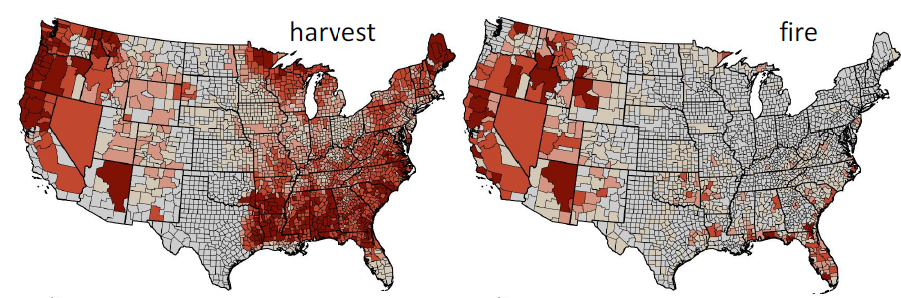
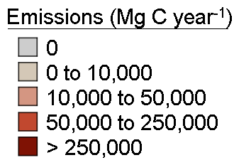
Figure 2. Average annual committed emissions attributed to forest fires and harvesting (Hagen et al.).

Conversion to other land use

Areas of forest converted to other land uses between 2006 and 2011 were identified using the National Land Cover Database (NLCD) for the years 2006 and 2011 (Jin et al., 2013). These products have a common 16-class land cover classification scheme that has been applied consistently across the United States at a spatial resolution of 30 meters. At the native 30-meter resolution, all converted pixels were identified as those that changed from NLCD-defined forest to agriculture, barren, or settlement. The 30-m map of converted areas was rescaled from the NLCD products into the 100-m common projection using the 3 x 3- pixel window approach and the fraction of converted area within this window was. The 100-m pixels were considered converted if more than half (> 4) of the original 30-m NLCD pixels were converted.

Wind damage

Areas of forest affected by wind damage caused by tornadoes or hurricanes were identified using data from the National Oceanic and Atmospheric Administration (NOAA) (NOAA Storm Prediction Center, http://www.spc.noaa.gov/gis/svrgis/, and the National Hurricane Center, http://www.nhc.noaa.gov/gis/). Paths and swath widths of all tornadoes occurring between 2006 and 2010 were translated into raster format. Hail and wind disturbances were excluded. Hurricane tracks where wind speeds exceeded 95 miles per hour (category 2 hurricane) were also included. The hurricane tracks were buffered to a symmetrical width of 100 km.

 

 

 

 

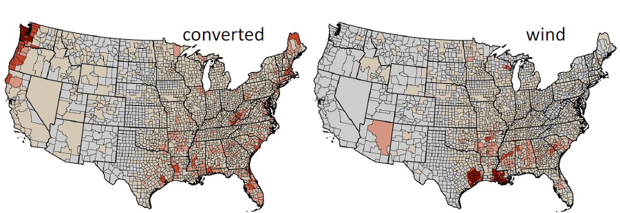
Figure 3. Average annual committed emissions attributed to wind and land conversion (Hagen et al.).

Drought damage

Areas affected by drought between 2006 and 2010 were identified using historical maps from Drought Monitor (data provided by the National Drought Mitigation Center (NDMC), the US Department of Agriculture (USDA) and the National Oceanic and Atmospheric Administration (NOAA); http://droughtmonitor.unl.edu/MapsAndData/GISData.aspx). The original Drought Monitor maps included five categories. Each category was assigned an integer value of 1 to 5, with increasing values corresponding to increasing drought intensity. Areas unaffected by drought were assigned a value of 0. The average drought intensity between 2006 and 2010 was calculated for each 100-m pixel.

Insect damage

Areas of insect disturbance were identified using annual aerial detection survey (ADS) data collected over forested lands by the USDA Forest Service (USDA Forest Service, Forest Health Protection and its partners, http://www.fs.usda.gov/detail/r2/forest-grasslandhealth/?cid=fsbdev3_041629). From these data, a disturbance severity metric was created based on number of trees with damage per acre surveyed. In future iterations of this work, these estimates could be improved by adjusting damage severity classes based on tree density. To create a single severity layer for the period of interest (2006-2010), for each 100-m pixel the number of trees damaged per acre across the time period was summed. The 100-m pixels were considered insect damaged if the insect damage intensity exceeded three trees per acre.

 

 

 

 

Figure 4. Average annual committed emissions attributed to insects and drought (Hagen et al.).

Co-occurrence of multiple damage types

In areas where multiple types of disturbance were identified within a 1-ha pixel, only one disturbance type was assumed to be driving the carbon loss. Disturbance type priority was set based on level of confidence in the data sets. The disturbance type priority varies across multiple iterations of our sensitivity analysis.

 

Creation of Net Carbon Flux Lookup Tables from FIA Plot Data

More than 141,000 records were extracted associated with re-measured permanent plots in the FIA database, where each extracted record represented a “condition” (i.e. domain(s) mapped on each plot using land use, forest type, stand size, ownership, tree density, stand origin, and/or disturbance history) of a measured plot at two points in time. From these records, changes were estimated in the above- and belowground carbon pools over time and a lookup table was created stratified by geographic region, forest type, disturbance type, and disturbance intensity. These average annual flux values per pool and per stratum were linked to spatial estimates of disturbance type and intensity derived from independent data (i.e., remote sensing-based estimates). Annual net carbon flux estimates per stratum represents a combination of gross removals and gross emissions (caused by disturbances) that occurred between the FIA measurement dates.

For the purposes of this analysis, CONUS was divided into three general geographic regions: North, South and West, following the divisions of Zheng et al. (2011) which were loosely based on USDA Forest Service FIA regions. Forest types in our analysis were defined as hardwood or softwood. The basis of our forest type classification was the 2006 National Land Cover Database (NLCD) (30-m resolution). The 30-m data were resampled to 100-m using the 3 x 3-pixel window approach described above. In this case, each 100-m pixel was assigned a value for percent hardwood and percent softwood. Hardwoods were defined as the deciduous forest class from the NLCD 2006 and softwoods as the evergreen forest class.

A similar stratification procedure was used for re-measurement plots where no disturbance occurred to create a lookup table of annual net carbon flux in undisturbed forests from above- and belowground biomass pools based on region, forest type, base carbon stock in 2005, and presence or absence of drought. FIA plots were assigned to the drought affected category if they had an average drought intensity of more than two between the years of measurement and to the drought free category if they had an average drought intensity of two or lower between the years of measurement.

No change was assumed for the standing dead carbon pool for undisturbed areas. For disturbed areas, changes were assumed and were related to the type of disturbance. During forest conversion from forest to agriculture or settlement, all dead carbon was assumed to be immediately emitted to the atmosphere. Over the long-term (100 years) following fire, insect, and wind disturbance, the carbon killed in the live pools (above and below) is emitted to the atmosphere (Russell et al., 2014).

 

Model description

A data-driven, spatially explicit framework was developed to account for carbon fluxes across US forest lands between 2005 and 2010. Initially, each pixel was identified as disturbed or undisturbed.

Next, for disturbed pixels, information from various geospatial data sets described above was used to assign a disturbance type and a disturbance severity. The methodology is described below.

 

Disturbed and Undisturbed Pixel Categorization.

Disturbance intensity and disturbance type were estimated for pixels disturbed between 2006 and 2010.

Identification of Disturbance Location

Information from all disturbance layers was used to categorize each pixel as disturbed or undisturbed. This includes information derived from the Hansen et al. (5) forest cover products (i.e. lateloss), insect damage intensity, fire burn severity, tornado and hurricane paths, and NLCD-based conversion maps. Pixels that were identified as being substantially disturbed in at least one of these five layers (i.e. maximum burn severity of at least 2 over the five years; insect damage total of at least 3 trees per acre over the five years; within a path of a hurricane or tornado between 2006 and 2010; identified as converted to agriculture or settlement in the NLCD layer between 2006 and 2011; or identified as forest loss in the Hansen data set were categorized as having been disturbed during the 2006-2010 time period.

Identification of Disturbance Type

Once a pixel was determined to have been disturbed, disturbance type was estimated using the same methodology described for determining disturbance location. Five data layers were provided as input in the determination: insect damage intensity, fire burn severity, tornado and hurricane paths, NLCD-based conversion maps, and the timberlands map. Relative intensity of insect damage and burn severity of a pixel, as well as its location within a converted area, tornado/hurricane path, or timberland area determined the assigned disturbance type. Pixels with multiple possible disturbance types were assigned a single disturbance type based on the relative assessed quality of the input data sets (and the resulting sensitivity to this assessment of relative quality was tested during the sensitivity assessment). Areas identified as experiencing lateloss in the Hansen forest cover data set but not appearing in other disturbance data layers were assigned to the harvest disturbance type (i.e. Harvest-RS).

Identification of Disturbance Intensity

After disturbance type for a pixel was identified, the disturbance intensity was determined using available information relevant to each disturbance type. Fire disturbance intensity was determined at three levels using Hansen forest cover lateloss and fire burn severity level (from the MTBS data set).

Insect disturbance intensity was determined at three levels using Hansen forest cover lateloss and insect damage per acre (from the Areal Detection Survey). Wind disturbance intensity was determined at two levels using Hansen forest cover lateloss. Areas determined to have been converted to agriculture or settlement were assumed to experience one uniform intensity. The areas identified as harvested (i.e. identified as lateloss in the Hansen Forest Cover data set, but are not in any other loss data set) were assumed to have experienced intense, or stand-replacement, harvest.

 

Carbon Flux Calculations

Gross carbon sequestration

Gross sequestration between 2005 and 2010 was calculated across the entire forest domain of 2005, regardless of presence of disturbance. The single exception to this was areas converted to other land use (i.e. agriculture, barren, or settlements) which were assumed to have been converted halfway through the time period and therefore accumulate carbon for 2.5 years instead of five. Gross sequestration was calculated based on initial 2005 stock, forest type, region, and presence/absence of drought using the lookup tables containing fractional change in carbon that were created from undisturbed FIA plot data. This process estimated carbon accumulation in the above- and belowground carbon pools, and these pools add together for total C accumulation per pixel because we assume no change in the dead and soil carbon pools in the absence of disturbance. In this analysis, carbon sequestration from background forest growth was treated the same as carbon sequestration from forest gains (e.g. afforestation or reforestation).

Net carbon flux

Net carbon flux was calculated in two separate ways depending on the pixel’s disturbance status. For undisturbed pixels, net carbon flux was equal to the gross sequestration. For pixels experiencing a disturbance between 2006 and 2010, net carbon flux was calculated based on initial 2005 stock, forest type, region, type of disturbance, and intensity of disturbance, using the lookup tables containing fractional change in carbon that were created from disturbed FIA plot data.

Gross carbon emissions

Gross carbon emissions within disturbed pixels were estimated as the net carbon flux minus gross sequestration. This assumes that the carbon accumulation rate within a disturbed pixel does not change after disturbance. Converted pixels, however, are assumed to stop accumulating carbon at the mean date of disturbance, which allows for 2.5 years of carbon accumulation, rather than five.

 

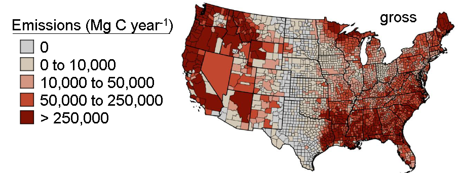
Figure 5.Gross carbon emissions in the US (Hagen et al.).

Logging-Non-spatial attribution of additional harvest carbon emissions

Timber harvest data for the US do not exist at scales finer than combined counties. The analysis presented assumes that forest cover change (Hansen et al., 2013) that is not associated with fire, wind, insect outbreak, or conversion to settlement, barren, or agriculture is harvested land that falls within designated timberland areas. This catch-all category is enhanced through comparison with the 2007 TPO data from the USFS. TPO data was used to estimate annual aboveground carbon flux from harvest at the combined county and state levels. Then our spatially resolved estimates for harvest within designated timberland areas were assumed to represent the spatially intensive, larger scale component of harvesting. The difference in carbon emission estimates at the state level between those derived from the TPO data and those derived from our spatially resolved estimates represent the less intensive, selective harvest component that is not easily observable in remote sensing imagery. Therefore, estimates of carbon flux from logging within the model framework come from a combined two-step approach:

1. Spatially explicit estimates of tree cover loss from disturbances larger than 1-ha (Hansen et al., 2013) were attributed to one of a list of causes (e.g. conversion, fire, insect, or wind) for which we have other, independent observations. Areas in timberlands identified as experiencing tree cover loss but that do not overlap with an independent attributable cause are assumed to be caused by harvest. The carbon flux associated with this logging activity was estimated using the same approach as other attributed causes: by combining average change in carbon stock estimates derived from the FIA plots disturbed by logging between re-measurement years with initial carbon stock estimates from the base carbon stock maps. Estimates of carbon flux generated in this step were named “spatially resolved logging flux estimates” (or Harvest-RS) and these estimates include changes to the above ground and below ground pools. The emissions committed to the atmosphere over the 100-year period following the logging event were calculated as the killed live (above and below ground) biomass minus the fraction of biomass stored in long-term wood products beyond 100 years.

Carbon flux from “spatially resolved” harvested areas was assumed to be intensive, resulting in above and belowground carbon loss rate determined in the FIA lookup table, typically around 80% over the five year period (the net result of a nearly complete loss of live carbon followed by regrowth). These harvested areas are assumed to lose 5% of the carbon in the dead pool in the five year period and no change in the soil carbon pool.

2. Carbon flux estimates generated from Step 1 above were then compared to state-wide carbon emissions estimates associated with logging derived from mill surveys compiled into the TPO database. To estimate carbon emissions from timber harvesting based on volumes reported in the TPO database, data were extracted based on the volume of roundwood products, mill residues and logging residues, separated by product class and detailed species group. The spatial scale of the data was the “combined county”, which represented the minimum reportable scale from the TPO dataset while retaining necessary confidentiality. Volumes were converted to biomass using oven-dry wood density information (Miles and Smith 2009). Timber harvesting emissions are complicated by the reality that changes in live biomass stocks in the forest occur at a single point in time while emissions, especially from derived wood products will continue for very many years. Both the initial categorization of biomass pools between residues and product classes, and the “committed emissions” were included which were considered to be all emissions expected to occur during the 100-years immediately after timber harvest.

Products were divided into seven classes, with Smith et al. (2006) used to determine fraction of carbon in primary wood products remaining either in end uses or in landfills 100 years after harvest. The TPO and Smith et al. (2006) classes were crosswalked as follows:

   Sawlog = Softwood/Hardwood Lumber (depending on species);

   Veneer = Softwood Plywood;

   Pulp = Paper;

   Composite = Oriented Strandboard

Fuelwood, posts/poles/pilings and miscellaneous were assumed fully emitted within the 100 year time period. Emissions from mill residues were considered equal to the summed mill residues from fuel byproducts, miscellaneous by-products and unused mill residues plus emissions from fiber byproducts. All fiber by-products were assumed to form pulp and to follow the emissions assumptions of pulp products. All logging residues were considered to be emissions to the atmosphere.

At the state-level, the average annual carbon emissions from above ground biomass associated with logging in Step 1 above is subtracted from the TPO estimates of carbon emissions associated with logging in 2007. The difference was assumed to represent all of the above ground carbon associated with logging occurring in areas too small to identify with 30-m remote sensing observations (i.e. Hansen et al., (2013)), which we call “spatially unresolved carbon emissions estimates” (or Harvest-TPO).

The ratio of above ground carbon emissions associated with harvest to below ground carbon emissions from harvest were calculated at the state level from the “spatially resolved carbon emissions estimates”. This state level above to below-ground ratio was then applied to the TPO emissions estimate at the combined county level. The combo county level maps of carbon emissions from harvest include a) the TPO 2007 estimates of above ground carbon associated with logging adjusted for long-term wood product storage and b) additional carbon emissions from below ground carbon using this above to below ground ratio.

Eidenshink, J., Schwind, B., Brewer, B., Zhu, Z-L. Quayle, B., and Howard, S. (2007). A project for monitoring trends in burn severity. Fire Ecology 3(1):3-21.

Hagen,S.C., N.L. Harris, S.S. Saatchi, T.R.H. Pearson, C.W. Woodall, S. Ganguly, G.M. Domke, B.H. Braswell, B.F. Walters, J. Jenkins, S. Brown, W. Salas, A. Fore, Y. Yu, R. Nemani, C. Ipsan, and K.R. Brown. Attribution of carbon emissions by disturbance type across forest land of the United States.  In prep.

Hansen, M.C., P.V. Potapov, R. Moore, M. Hancher, S.A. Turubanova, A. Tyukavina, D. Thau, S.V. Stehman, S. J. Goetz, T.R. Loveland, A. Kommareddy, A. Egorov, L. Chini, C.O. Justice, J. R.G. Townshend (2013). High-resolution global maps of 21st-century forest cover change. Science 342(6160):850–853.

Healey, S. P., Patterson, P. L., Saatchi, S., Lefsky, M. A., Lister, A. J., & Freeman, E. A. (2012). A sample design for globally consistent biomass estimation using lidar data from the Geoscience Laser Altimeter System (GLAS). Carbon balance and management, 7(1), 1-9.

Lefsky, M. A. (2010). A global forest canopy height map from the Moderate Resolution Imaging Spectroradiometer and the Geoscience Laser Altimeter System. Geophysical Research Letters, 37(15).

Jin, S., Yang, L., Danielson, P., Homer, C., Fry, J., and Xian, G. (2013). A comprehensive change detection method for updating the National Land Cover Database to circa 2011. Remote Sens Environ 132:159-175.

Miles PD, Smith WB (2009) Specific gravity and other properties of wood and bark for 156 tree species found in North America. USDA For Ser North Res Stn Res Note NRS-38, Newtown Square, PA. 35p.

Nelson, Mark D.; Liknes, Greg C.; Butler, Brett J. 2010. Map of forest ownership in the conterminous United States Scale 1:7,500,000. Res. Map NRS-2. Newtown Square, PA: U.S. Department of Agriculture, Forest Service, Northern Research Station.

Russell, Matthew B.; Woodall, Christopher W.; Fraver, Shawn; D'Amato, Anthony W.; Domke, Grant M.; Skog, Kenneth E. 2014. Residence times and decay rates of downed woody debris biomass/carbon in eastern US forests. Ecosystems. 17(5): 765-777.

Saatchi, S.S, Harris, N.L., Brown, S., Lefsky, M., Mitchard, E.T.A., Salas, W., Zutta, B.R., Buermann, W., Lewis, S.L., Hagen., S., Petrova, S., White, L., Silman, M., and Morel, A.  (2011). Benchmark map of forest carbon stocks in tropical regions across three continents. Proc Natl Acad Sci U S A 108(24):9899-9904. doi: 10.1073/pnas.1019576108.

Saatchi, Sassan.S., Alexander Fore, Yifan Yu, Christopher Woodall , Sangram Ganguly, Rama Nemani, Gong Zhang, Steven C. Hagen, Nancy L. Harris, Sandra Brown, Richard Birdsey, Kristofer D. Johnson, Liang Xu, Yan Yang, William. Salas, National carbon inventory of the US forestlands from space. In prep for Remote Sensing of Environment.

Smith, J.E., Heath, L.S., Skog, K.E., Birdsey, R.A. (2006). Methods for calculating forest ecosystem and harvested carbon with standard estimates for forest types of the United States. USDA For Ser North Res Stn Gen Tech Rep NE-243, Newtown Square, PA. 216 p.

Smith, J.E., and Heath, L.S. (2002) A model of forest floor carbon mass for United States forest types.

USDA For Ser North Res Stn Res Paper NE-722, Newtown Square, PA. 37 p.

USDA Forest Inventory and Analysis National Program (FIA), Resource Planning Act (PRA), Maps of Timberland, 2007 http://www.fia.fs.fed.us/tools-data/maps/2007/index.php.

Woodall, C.W.; Walters, B.F.; Oswalt, S.N.; Domke, G.M.; Toney, C.; Gray, A.N. 2013. Biomass and carbon attributes of downed woody materials in forests of the United States. Forest Ecology and Management. 305: 48-59.

Woodall, C.W. et al. In Press. Dead wood net carbon flux in forests of the eastern United States. Oecologia.

Zheng D, Heath L.S., Ducey, M.J., Smith,  J.E. (2011) Carbon changes in conterminous US forests associated with growth and major disturbances: 1992–2001. Environ Res Lett 6:014012.doi:10.1088/1748-9326/6/1/014012.