Documentation Revision Date: 2016-11-14
Data Set Version: V1
Summary
These measurements are one part of an innovative multi-instrument remote sensing payload flown for the CARVE investigation.
There are 4 data files in netCDF (*.nc) format, one for each year of CARVE campaign flights, with this data set.
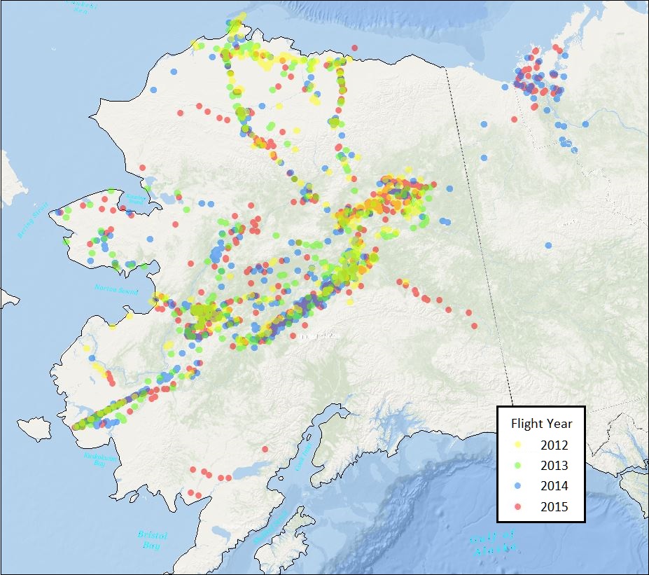
Figure 1: Locations of CARVE flask air samples from flights between 2012-2015
Citation
Sweeney, C., J.B. Miller, A. Karion, S.J. Dinardo, and C.E. Miller. 2016. CARVE: L2 Atmospheric Gas Concentrations, Airborne Flasks, Alaska, 2012-2015. ORNL DAAC, Oak Ridge, Tennessee, USA. http://dx.doi.org/10.3334/ORNLDAAC/1404
Table of Contents
- Data Set Overview
- Data Characteristics
- Application and Derivation
- Quality Assessment
- Data Acquisition, Materials, and Methods
- Data Access
- References
Data Set Overview
Project: Carbon in Arctic Reservoirs Vulnerability Experiment (CARVE)
The Carbon in Arctic Reservoirs Vulnerability Experiment (CARVE) is a NASA Earth Ventures (EV-1) investigation designed to quantify correlations between atmospheric and surface state variables for Alaskan terrestrial ecosystems through intensive seasonal aircraft campaigns, ground-based observations, and analysis sustained over a 5-year mission. CARVE collected detailed measurements of greenhouse gases on local to regional scales in the Alaskan Arctic and demonstrated new remote sensing and improved modeling capabilities to quantify Arctic carbon fluxes and carbon cycle-climate processes. CARVE science fills a critical gap in Earth science knowledge and satisfies high priority objectives across NASA’s Carbon Cycle and Ecosystems, Atmospheric Composition, and Climate Variability & Change focus areas as well as the Air Quality and Ecosystems elements of the Applied Sciences program. CARVE data also complements and enhances the science return from current NASA and non-NASA sensors.
Related Data:
A full list of CARVE data products is available at: https://carve.ornl.gov/dataproducts.html
Data Characteristics
Spatial Coverage: CARVE flights over the Alaskan and Canadian Arctic
Spatial Resolution: Point measurements
Temporal Coverage: 20110329 - 20151112
Temporal Resolution: The instruments were deployed on periodic flights during the growing season (approx. March – November). Measurements were initiated by the aircraft pilot at scheduled times coinciding with overflight of an area of interest, or when interesting geophysical conditions were encountered. A minimum of 12 flask samples were collected per flight.
Study Area (coordinates in decimal degrees)
|
Site |
Westernmost Longitude |
Easternmost Longitude |
Northernmost Latitude |
Southernmost Latitude |
|
Alaska and Canadian Arctic |
-167.4810 |
-104.3540 |
71.4985 |
35.2004 |
Data File Information
All data are stored in NetCDF (*.nc) version 4 file format. Each file provides measurements of dry mole fractions of atmospheric CO2, CH4, CO, H2, N2O, and SF6 acquired over one year of CARVE flights.
Table 1: CARVE file naming convention. Example file name: carve_Flask_L2_b23_20121001_20160807204049.nc
|
Name element |
Example value |
Units |
|
Project name |
carve |
|
|
Instrument |
Flask |
|
|
Processing level |
L2 |
|
|
Build ID |
b23 |
|
|
Flight date start |
20121001 |
yyyymmdd |
|
Processing date and time |
20160807204049 |
yyyymmddhhmmss |
Data variables
Each file contains 14 geolocation and ancillary variables and 69 science measurement variables described in Table 2.
Table 2. Data variables in each netCDF file. Fill value or missing data were set to -999.9 for all variables.
|
Variable name |
Description |
Units |
|
Geolocation and ancillary measurements |
|
|
|
center_lat |
latitude |
decimal degrees North |
|
center_lat_standard_error |
latitude standard error |
decimal degrees North |
|
center_lon |
longitude |
decimal degrees East |
|
center_lon_standard_error |
longitude standard error |
decimal degrees East |
|
height |
height of aircraft above ground |
meters |
|
height_standard_error |
height standard error |
meters |
|
geolocation_qc |
geolocation status flag |
0 = Success, 1 = Error |
|
time |
time of sample collection |
seconds since 1980-1-6 0:0:0 |
|
elevation |
surface elevation |
meters |
|
event_number |
NOAA database event number |
|
|
intake_height |
sample intake height |
meters |
|
flask_id |
sample container ID |
|
|
sample_method |
sample collection method |
|
|
site_code |
sample site code |
|
|
Science measurements |
|
|
|
benz |
benzene (C6H6) |
parts per trillion (ppt) * |
|
brfm |
bromoform (CHBr3) |
ppt |
|
c2f6 |
hexafluoroethane (CF3CF3) |
ppt |
|
c2h2 |
ethyne (acetylene; C2H2) |
ppt |
|
c2h4 |
ethene (ethylene; C2H4) |
ppt |
|
c2h6 |
ethane (C2H6) |
ppt |
|
c3h6 |
propene (propylene; C3H6) |
ppt |
|
c3h8 |
propane (C3H8) |
ppt |
|
ccl4 |
carbon tetrachloride (tetrachloromethane; CCl4) |
ppt |
|
cf4 |
carbon tetraflouride (tetrafluoromethane; CF4) |
ppt |
|
ch2brcl |
bromochloromethane (CH2BrCl) |
ppt |
|
ch3i |
methyl iodide (CH3I) |
ppt |
|
ch4 |
methane (CH4) |
parts per billion (ppb) * |
|
chlf |
chloroform (CHCl3) |
ppt |
|
co |
carbon monoxide (CO) |
ppb |
|
co2 |
carbon dioxide (CO2) |
parts per million (ppm) * |
|
co2c13 |
d13C of CO2 |
ppm |
|
co2c14 |
d14C of CO2 |
ppm |
|
co2o18 |
d18O of CO2 |
ppm |
|
cs2 |
carbon disulfide (CS2) |
ppt |
|
dibr |
dibromomethane (CH2Br2) |
ppt |
|
dicl |
dichloromethane (CH2Cl2) |
ppt |
|
f112 |
CFC-112 (CCl3CClF2) |
ppt |
|
f113 |
CFC-113 (CCl2FCClF2) |
ppt |
|
f114 |
CFC-114 and CFC-114a (ClF2CCF2Cl) |
ppt |
|
f115 |
CFC-115 (CClF2CF3) |
ppt |
|
f11a |
CFC-11 (ion 101; CCl3F) |
ppt |
|
f11b |
CFC-11 (ion 103; CCl3F) |
ppt |
|
f124 |
HCFC-124 (CHClFCF3) |
ppt |
|
f125 |
HFC-125 (CHF2CF3) |
ppt |
|
f13 |
CFC-13 (CClF3) |
ppt |
|
f134 |
HFC-134 (CHF2CHF2) |
ppt |
|
f134a |
HFC-134a (CH2FCF3) |
ppt |
|
f141b |
HCFC-141b (CH3CCl2F) |
ppt |
|
f142b |
HCFC-142b (CH3CF2Cl) |
ppt |
|
f143a |
HFC-143a (CH3CF3) |
ppt |
|
f152a |
HFC-152a (CH3CHF2) |
ppt |
|
f160 |
chloroethane (CH3CH2Cl) |
ppt |
|
f227e |
HFC-227ea (CF3CHFCF3) |
ppt |
|
f23 |
HFC-23 (CHF3) |
ppt |
|
f236fa |
HFC-236fa (CF3CH2CF3) |
ppt |
|
f32 |
HFC-32 (CH2F2) |
ppt |
|
f365m |
HFC-365mfc (CH3CF2CH2CF3) |
ppt |
|
fc12 |
CFC-12 (CCl2F2) |
ppt |
|
h1211 |
bromochlorodifluoromethane (halon 1211; CBrClF2) |
ppt |
|
h1301 |
bromotrifluoromethane (halon 1301; CF3Br) |
ppt |
|
h2 |
hydrogen (H2) |
ppb |
|
h2402 |
dibromotetrafluoroethane (halon 2402; CBrF2CBrF2) |
ppt |
|
hf133a |
HCFC-133a (CH2ClCF3) |
ppt |
|
hf21 |
HCFC-21 (CHCl2F) |
ppt |
|
hf22 |
HCFC-22 (CHF2Cl) |
ppt |
|
ic4h10 |
i-butane (i-C4H10) |
ppt |
|
ic5h12 |
i-pentane (i-C5H12) |
ppt |
|
mcfa |
methyl chloroform (ion 97; CH3CCl3) |
ppt |
|
mebr |
methyl bromide (CH3Br) |
ppt |
|
mecl |
methyl chloride (CH3Cl) |
ppt |
|
n2o |
nitrous oxide (N2O) |
ppb |
|
nc4h10 |
n-butane (n-C4H10) |
ppt |
|
nc5h12 |
n-pentane (n-C5H12) |
ppt |
|
nc6h14 |
n-hexane (n-C6H14) |
ppt |
|
nf3 |
nitrogen trifluoride (NF3) |
ppt |
|
ocs |
carbonyl sulfide (COS) |
ppt |
|
p218 |
perfluoropropane (C3F8) |
ppt |
|
pce |
tetrachloroethylene (C2Cl4) |
ppt |
|
sf6_ccgg |
sulfur hexafluoride (SF6) |
ppt |
|
sf6_hats |
sulfur hexafluoride (SF6) |
ppt |
|
so2f2 |
sulfuryl fluoride (SO2F2) |
ppt |
|
tce |
trichloroethylene (C2HCl3) |
ppt |
|
tol |
toluene (C7H8) |
ppt |
* parts per million – ppm – micromol of gas per mol of dry air – 10-6
parts per billion – ppb – nanomol of gas per mol of dry air – 10-9
parts per trillion – ppt – picmol of gas per mol of dry air – 10-12
The netcdf files also include a QC flag for each analyte. For example, the benzene ratio QC flag is “benz_ratio_status”. The flag values are the same for all analytes and are provided in Table 3.
Table 3. QC flag value descriptions
|
QC Flag |
Flag Meaning |
Description |
|
1 |
Valid |
|
|
2 |
Preliminary |
Sample measurement is preliminary and has not yet been carefully examined by the PI |
|
3 |
Deselected |
Sample measurement is likely valid but does not meet selection criteria determined by the goals of the CARVE investigation |
|
4 |
Rejected |
Obvious problems during collection or analysis |
Calibration:
All measurements are reported as dry air mole fractions on their respective World Meteorological Organization (WMO) standard scales:
- NOAA 2004 CO standard scale (see Novelli et al., 1991)
- NOAA 2007 CO2 standard scale (see Zhao and Tans, 2006)
- NOAA 2004 CH4 standard scale (see Dlugokencky et al., 2005)
- NOAA 2004 CMDL H2 standard scale (Novelli et al., 1999)
- NOAA 2006A N2O standard scale (Hall et al., 2007)
- NOAA 2006 SF6 standard scale (Hall et al., 2011)
Application and Derivation
These data files contain dry mole fractions of CO, CO2, CH4, H2, N2O, and SF6 measured from whole air samples collected during CARVE flights between March and November of 2012 to 2015. These data complement high-frequency gas concentration observations from the Fourier transform spectrometer and cavity ring-down spectroscopy instruments aboard CARVE flights.
The CARVE project was designed to collect detailed measurements of important greenhouse gases on local to regional scales in the Alaskan arctic and demonstrate new remote sensing and improved modeling capabilities to quantify Arctic carbon fluxes and carbon cycle-climate processes. The CARVE data provide insights into Arctic carbon cycling that may be useful in numerous applications.
Quality Assessment
Table 4. Repeatability of gas detection was determined as 1 standard deviation of ~20 aliquots of natural air measured from a standard cylinder.
|
Gas |
Average Repeatability |
|
CO |
UV Resonance fluorescence: +/- 0.4 ppb (Gerbig et al., 1999) |
|
CO2 |
+/- 0.03 ppm (Conway et al., 1994) |
|
CH4 |
+/- 1.2 ppb (Dlugokencky et al., 1994) |
|
H2 |
+/- 0.4 ppb (Novelli et al., 1999) |
|
N2O |
+/- 0.26 ppb (Dlugokencky et al., 2009) |
|
SF6 |
+/- 0.03 ppt (Dlugokencky et al., 2009) |
Data Acquisition, Materials, and Methods
CARVE Flights
These data represent one part of the data collected by the Carbon in Arctic Reservoirs Vulnerability Experiment (Miller & Dinardo, 2012). A C-23 Sherpa aircraft made frequent flights out of Fairbanks, Alaska between March and November over multiple years, observing the spring thaw, summer draw-down, and fall refreeze of the Arctic growing season. Flights concentrate observations on three study domains: the North Slope, the interior, and the Yukon River valley. North Slope flights cover regions of tundra and continuous permafrost and were anchored by flux towers in Barrow, Atqasuk, and Ivotuk. Flights to Prudhoe Bay characterize the CO2 and CH4 emissions from oil and natural gas processing plants. Flights over interior Alaska sample discontinuous permafrost, boreal forests, and wetlands. A complete list of CARVE flights can be found at: https://carve.ornl.gov/flights.html. Flight paths and atmospheric gas concentrations for CARVE surveys can be visualized through the CARVE Flight Data Visualization Tool (http://carve.ornl.gov/visualize) and are illustrated in Figure 2.
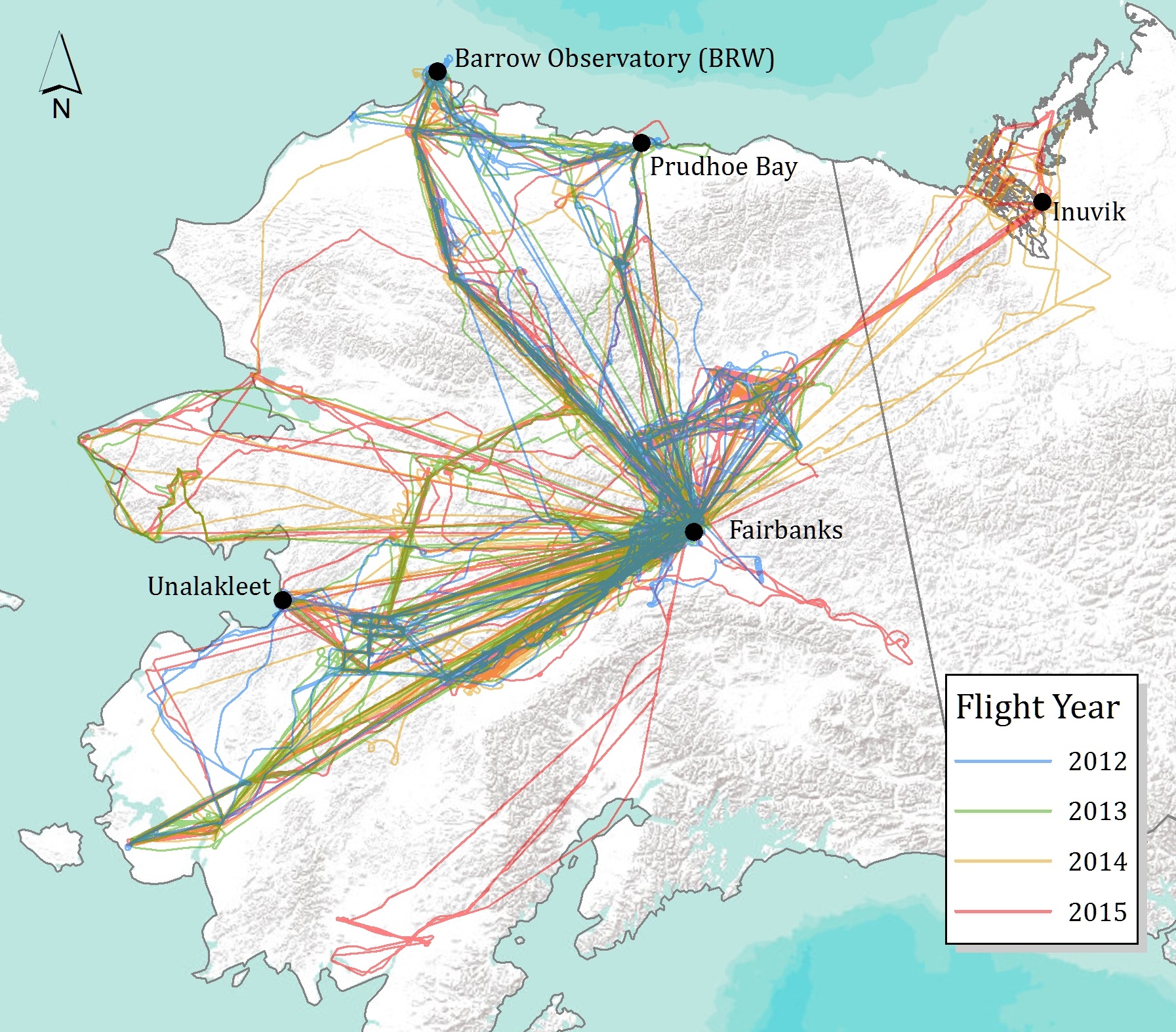
Figure 2. CARVE flights during 2012-2015 delivered measurements over continuous and discontinuous permafrost regimes.
The CARVE aircraft carried a remote sensing and atmospheric sampling payload consisting of the following instruments: a Fourier transform spectrometer (FTS), and an in situ gas analyzer suite (ISGA) with a gas analyzer and PFP sampling system (see https://carve.ornl.gov/documentation.html). All instruments were controlled by a master computer system (Data Acquisition and Distribution System, DADS). Data were logged and UTC time stamped at 1 second intervals. DADS also recorded GPS data (Lat, Lon, elevation), aircraft pitch, roll, and yaw, as well as basic meteorological data from onboard instruments.
Flask air sampling system
This data set includes measurements from discrete air samples captured by the flask sampling system on board the aircraft. The two air-sampling devices, the Programmable Flask Package (PFP) and Programmable Compressor Package (PCP) systems, are used routinely on aircraft as part of the NOAA/ESRL Global Monitoring Division’s Carbon Cycle and Greenhouse Gases network (Sweeney et al., 2013).
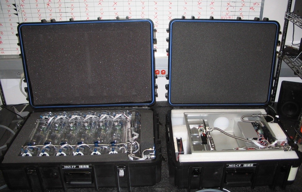
Figure 3. Flask sampling system for aircraft measurements. Left: Programmable Flash Package (PFP) containing 12 flasks. Right: Programmable Compressor Package (PCP) containing pumps for pressurizing the flasks. (Image courtesy: http://www.esrl.noaa.gov/gmd/ccgg/aircraft/sampling.html)
A typical sampling routine uses one PCP and one or more PFP(s) that are pre-programmed with a flight-specific sampling plan of target altitudes for each sample. Sampling is timed to coincide with the overflight of a ground site of interest, or when interesting geophysical conditions are encountered. A map of flask sample locations is depicted in Figure 1. The PCP is connected to an LED display that communicates target sampling altitudes to the pilot. The pilot maintains the aircraft at a consistent altitude for the duration of each sample collection, typically under 40 seconds. For each sample, the inlet line and compression manifold are flushed with about 5 liters of ambient air. Valves on both ends of the current flask are then opened and the flask is flushed with about 10 more liters of ambient air to displace the dry, low CO2 fill gas with which the flasks are shipped. The sample flush air is measured by a mass flow meter to ensure that a sufficient volume passes through the manifold and flask before the downstream valve is closed and pressurization begins. Sample flush volumes and fill pressures during sampling are recorded by the data logger, along with ambient temperature, pressure, and relative humidity. GPS position and time stamp are also recorded with each sample.
Gas detection
- Quantities of CO2 in flask air samples were detected using a non-dispersive infrared analyzer and reported in parts per million (ppm). Because detector response is non-linear in the range of atmospheric levels, ambient samples are bracketed during analysis by a set of reference standards used to calibrate detector response.
- CH4 was isolated from constituent gases through gas chromatography and quantified with flame ionization detection. Measurements are reported in parts per billion (ppb).
- CO was isolated from constituent gases with gas chromatography and detected by resonance fluorescence at ~150 nm, or by reaction with HgO to produce mercury and detection through Hg resonance absorption, and reported in ppb.
- H2 was isolated using gas chromatography, reacted with HgO, and detected through Hg resonance absorption. H2 quantities are reported in ppb.
- The N2O and SF6 sample components were isolated using gas chromatography and quantified with electron capture detection. N2O and SF6 are reported in ppb and parts per trillion (ppt), respectively.
Data Access
These data are available through the Oak Ridge National Laboratory (ORNL) Distributed Active Archive Center (DAAC).
CARVE: L2 Atmospheric Gas Concentrations, Airborne Flasks, Alaska, 2012-2015
Contact for Data Center Access Information:
- E-mail: uso@daac.ornl.gov
- Telephone: +1 (865) 241-3952
References
Conway, T.J., et al. (1994). Evidence for interannual variability of the carbon cycle from the National Oceanic and Atmospheric Administration/Climate Monitoring and Diagnostics Laboratory Global Air Sampling Network, J. Geophys. Res., 99, 22,831–22,855.
Dlugokencky, E.J., L.P. Steele, P.M. Lang, K.A. Masarie (1994). The growth rate and distribution of atmospheric methane, J. Geophys. Res., 99, 17,021–17,043.
Dlugokencky, E.J., R.C. Myers, P.M. Lang, K.A. Masarie, A.M. Crotwell, K.W. Thoning, B.D. Hall, J.W. Elkins, and L.P. Steele (2005). Conversion of NOAA CMDL atmospheric dry air methane mole fractions to gravimetrically-prepared standard scale, J. Geophys. Res., 110, D18306 doi: 10.1029/2005JD006035
Dlugokencky, E. J., et al. (2009). Observational constraints on recent increases in the atmospheric CH4 burden, Geophys. Res. Lett., 36, L18803, doi:10.1029/2009GL039780
Gerbig, C., S. Schmitgen, D. Kley, A. Volz-Thomas, K. Dewey, D. Haaks (1999). An improved fast-response vacuum-UV resonance fluorescence CO instrument, J. Geophys. Res. 104, 1699 –1704.
Hall, B.D., G.S. Dutton, and J.W. Elkins (2007). The NOAA nitrous oxide standard scale for atmospheric observations, J. Geophys. Research, 112, D09305, doi:10.1029/2006JD007954
Hall, B.D., G.S. Dutton, D.J. Mondeel, J.D. Nance, M. Rigby, J.H. Butler, F.L. Moore, D.F. Hurst, and J.W. Elkins (2011). Improving measurements of SF6 for the study of atmosphere transport and emissions, Atmos. Meas. Tech. Discuss., 4, 4131-4163.
Miller, C.E., and S. J. Dinardo, "CARVE: The Carbon in Arctic Reservoirs Vulnerability Experiment," Aerospace Conference, 2012 IEEE, Big Sky, MT, 2012, pp. 1-17. doi: 10.1109/AERO.2012.6187026
Novelli, P. C., Elkins, J. W., and Steele, L. P. (1991). The development and evaluation of a gravimetric reference scale for measurements of atmospheric carbon monoxide, J. Geophys. Res.-Atmos., 96, 13109–13121, doi:10.1029/91jd01108
Novelli, P.C., P.M. Lang, K.A. Masarie, D.F. Hurst, R. Myers, J.W. Elkins (1999). Molecular hydrogen in the troposphere: Global distribution and budget, J. Geophys. Res. 104, 30,427-30,444.
Zhao, C., and P.P. Tans (2006). Estimating uncertainty of the WMO Mole Fraction Scale for carbon dioxide in air, J. Geophys. Res. 111, D08S09, doi: 10.1029/2005JD006003